![]()
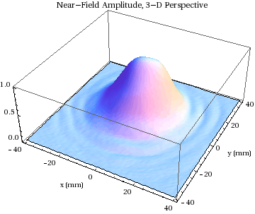
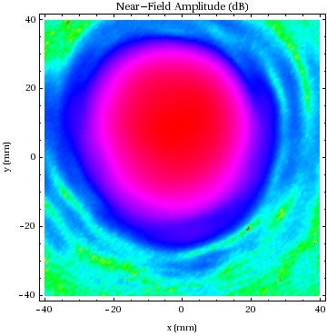
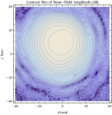
The data analyzed here are from Band 9 Scan 103, Beams 1 and 2,
in the linear combination (Beam1 - i Beam2)/2. The following three
plots show the near - field amplitude in 3-D perspective, then in the
form of a color density plot and as a contour plot. For the latter
the chosen contour levels are at (0, -3, -6, -9, ...) dB, with the peak
amplitude having been normalized to unity.
![]()
![]()
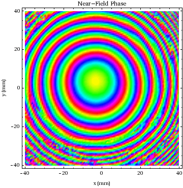
Now a plot of the near - field phase:
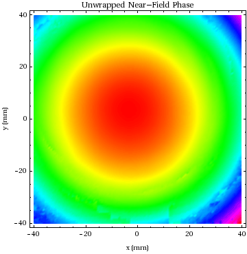
The following is a plot of the near - field phase after having
been unwrapped using an algorithm due to T. J. Flynn. See
Cennis C. Ghiglia and Mark D. Pritt, Two-Dimensional Phase
Unwrapping: Theory, Algorithms, and Software, Wiley, New York,
1998. The C code of Appendix A9 was used here. The original
publication the algorithm is (T. J. Flynn, JOSA A, 14 (1997) 2692 - 2701).
I call up the C code from within Mathematica. The run time
is ordinarily on the order of a few seconds.
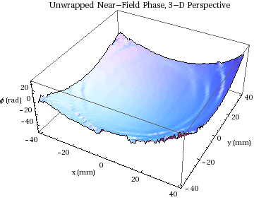
Here is a 3-D perspective plot of the unwrapped phase. The
only apparent problems in the unwrapping are near the edges :
![]()
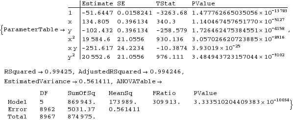
The following table gives the result of a linear least - squares
fit to the unwrapped phase. Here I fit for a constant term, the
x- slope, y- slope, and coefficients of ![]() , terms.
, terms.
Internally, the (x,y) units are meters, so here, e.g, the fitted x- slope
is 134.805 radians/meter with a standard error of 0.396 rad/m.
![]()
The NSI Band 9 Scan 103 measurements were taken over a 108×108
point grid. The (x,y)=(0,0) coordinate origin is located midway
between the central grid points. To achieve an effective 53.5 grid
point shift of origin in each coordinate I do a pre - FFT cyclic
leftward rotation by 53 grid units; then, post - FFT, I apply a phase
shift Exp(-i π (u Δx+v Δy)), to achieve the additional one - half
pixel shifts of origin. I could equally well have omitted the pre - FFT
cyclic shift and multiplied post - FFT by a factor Exp(-2 i π 53.5 (u Δx+v Δy)),
to thereby achieve the full shift of origin in just a single step.
I chose to zero pad to 512×512, same as NSI. However, I can
zero - pad to any desired size, even or odd parity, since Mathematica
has fast built - in algorithms for the discrete Fourier transform
for arbitrary n (even including prime n).
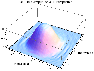
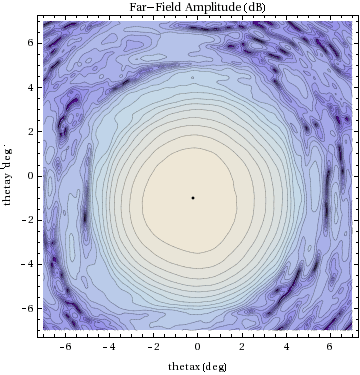
Here are plots of the computed far - field amplitude :
![]()
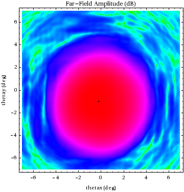
I use ![]() to denote the computed first moments of the
to denote the computed first moments of the
far - field amplitude distribution. This location is indicated
by the dot in the above figure and the one below.
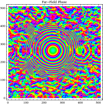
Here is a plot of the far - field phase, showing many phase
wraps and considerable noise.
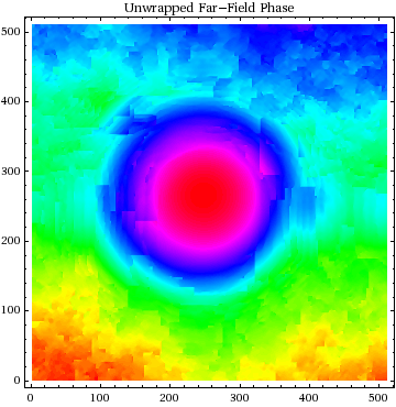
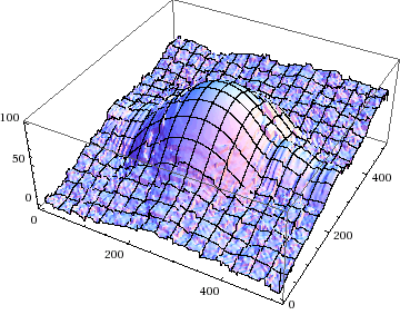
Below is an attempt at unwrapping the computed far - field
phase. The result looks OK over the central region of the beam,
where indeed several wraps were apparent, but once into the
sidelobes there are evident 2π n mistakes in the unwrapped result.
In this case, a 3-D perspective plot shows a better
picture of the result of the unwrapping algorithm. Again, the
ordinate is radians of phase.
The following table shows the the result of a linear
least - squares fit to the unwrapped far - field phase. Here
I have fit for a constant term and the coefficients of the ![]()
![]() and
and ![]() terms. The fit is to all the data
terms. The fit is to all the data
within a radius of 3.58° about ![]() ,
, ![]() ), and here I have weighted
), and here I have weighted
by amplitude.
![]()

From the fit I derive (x,y,z) offsets, in the frame of the
nominal beam - and a corresponding phase efficiency - which
are in reasonable accord with the results from Richard' s
spreadsheet. Fitting by weighted linear - least squares to
the unwrapped phase, and weighting the data by amplitude,
yields a phase efficiency essentially identical to that given by
Richard's efficiency maximization procedure.
![]()
![]()
![]()
![]()
![]()
![]()