Rotation Curve and Mass Decomposition for the Edge-on spiral galaxy UGC711

21-cm HI data from the Very Large Array (VLA) and optical R- and B- band data from the WIYN telescope are presented for the superthin galaxy UGC 711. An HI rotation curve is derived with two different methods, to determine which is the more accurate in the case of an edge-on galaxy. Beam smearing is taken into account and the mass contribution from the stars, gas and halo are determined by deriving equations for each of the components V_total²= V_stars² + V_gas² + V_halo² , and scaling the mass to light ratio and dark halo parameters for a good fit to the observed rotation curve.

Superthin galaxies are edge-on spiral galaxies that have a low surface brightness (LSB). Their edge-on orientation makes them fascinating to study, giving another perspective of spiral galaxies and allowing us to view galaxies which we would not be able to see face-on. One interesting property of superthin galaxies is that they exhibit a slowly rising rotation curve (Matthews, 1999). At the outermost measured point they are often still rising. The contribution of the stellar disk, even if scaled to its maximum possible value cannot explain the observed curve in the inner parts, unlike with high surface brightness (HSB) galaxies. This means that the stellar and gas components contribute little to the mass inferred from the rotation curve, helping to put constraints on the amount of dark matter in a galaxy (Swaters, et al, 2000).

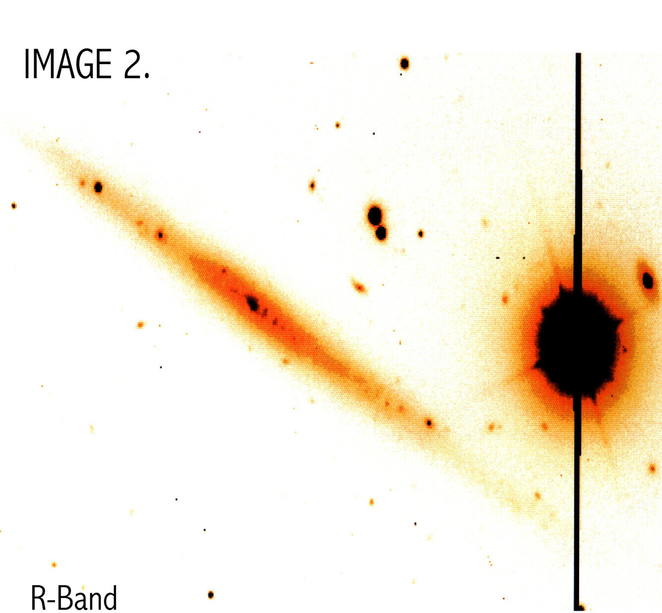
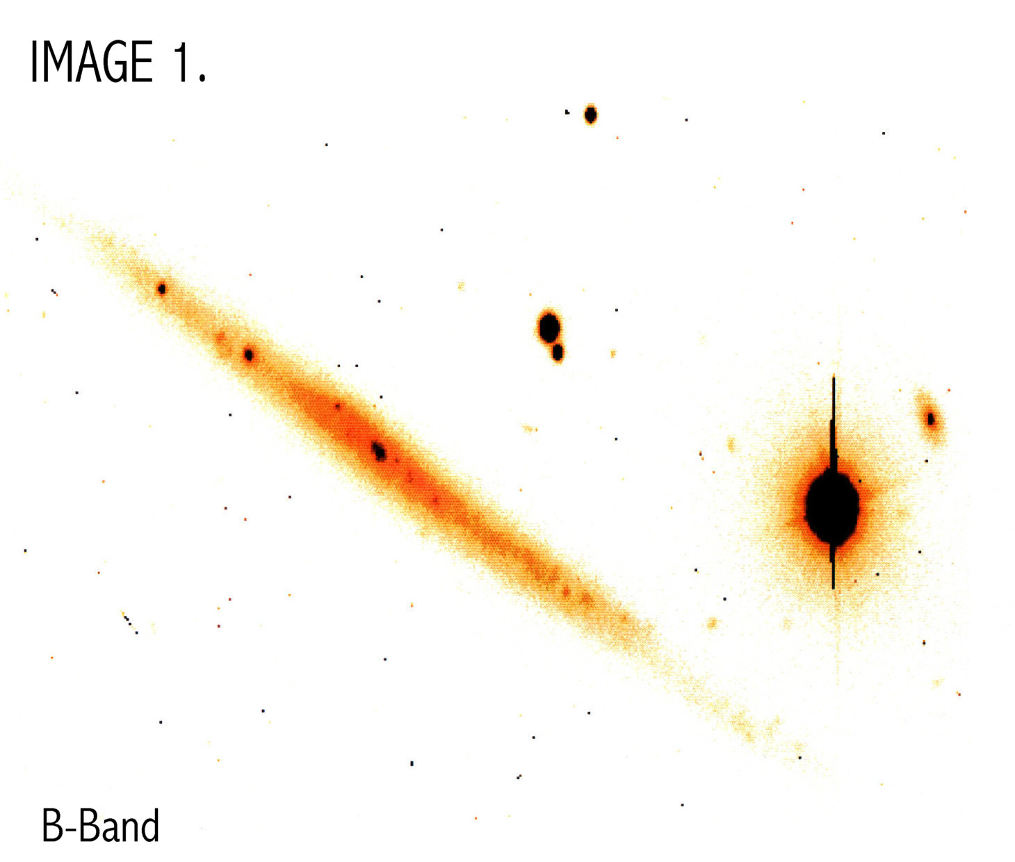
Lynn Matthews provided flatfielded B- and R- band images of UGC 711 taken with the WIYN telescope on Kitt Peak (IMAGES 1 &2).

The B-band exposure time was 900s and the R-band was 750s. These images were read into IRAF and are called U711R.fitsand U711B.fits. In IRAF I used procedures to carry out some basic editing. I subtracted the sky background by taking sample boxes of the sky background around and near the galaxy using the task imstat, which told me the mean sky flux for the box. Then I used imarith to subtract the average number of counts from the entire image. Using imexamin I checked sources to evaluate if they were foreground stars that should be removed. I removed the large, bright foreground star using imedit, and removed other foreground stars near the outer edges of the galaxy. I also removed cosmic rays with this procedure. These edited images are called test.Bremnsky2.fits and test.Rremnsky2.fits, for B and R band respectively. The center of the galaxy was then determined by eye, changing the contrast level in the image until the brightest central pixel was determined. To find ellipticity, position angle, diameter, and instrumental magnitude, I used a procedure called ellipse. I entered values for galaxy center, ellipticity, position angle, diameter, and number of ellipses into geompar, and then ran ellipse. Table 1 shows the values I used for the R- and B-band images.
 

Table 1.

R-BAND
Center	Ellipticity	Position Angle	Diameter	Number of Ellipses
x=996.10 y=1047.66	0.9	61	610	max=610 i=300sm=20
B-BAND
x=987.5 y=1052.5	0.9	61	610	max=610 i=300sm=20

To calculate the instrumental magnitudes I then converted the ellipses into apertures by first using elapert, which reads ellipse files into polyphot. Then I ran polyphot, which generates a .ply file of the instrumental magnitude within each aperture. Using a zeropoint magnitude of 26 the B-band instrumental magnitude is 16.24 and the R-band is 14.633. These were then converted into true apparent magnitudes using photometric solutions determined from standard stars (EQUATIONS 1 and 2):
 

Equation 1.

B-Mag = b0 - [bx (xb-1) + b +bc [(b-r) - (xb-1)brx]

Where b0=zero point= -1.749396

bx= extinction coefficient= 0.3663924

brx= b-r extinction coefficient= 0.1643354

bc= color term= 0.00601

xb= airmass= 1.209239

b = B-band instrumental magnitude = 16.24

b-r= instrumental B-R color= 16.24- 14.633= 1.606

Equation 2.

B-R Mag= br0 - [brx (xr-1)] +(b-r) +brc [(b-r) - brx(xr-1)]

Where br0= zero point= -0.6383474

brc= .03705169

xr= 1.187522

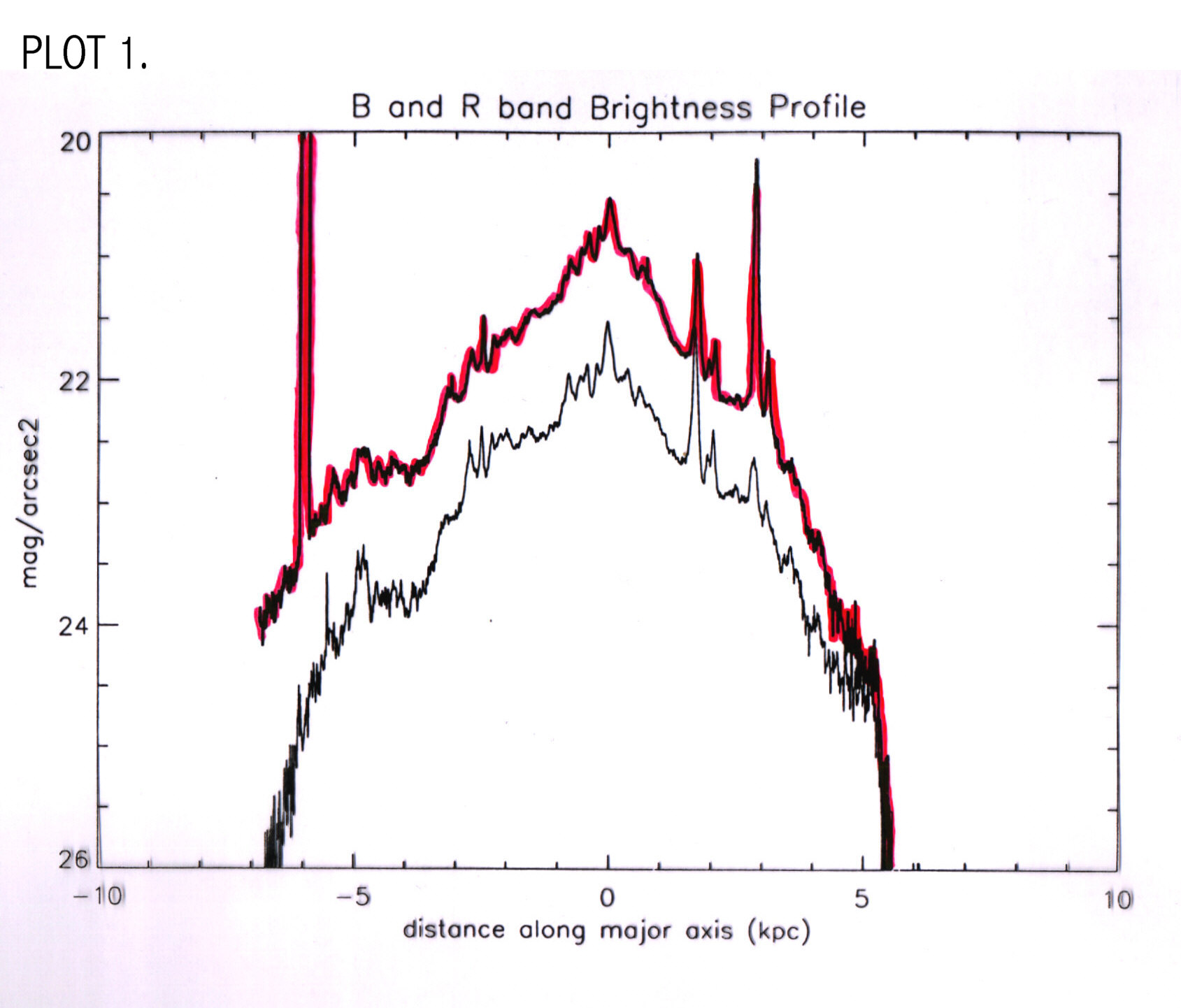
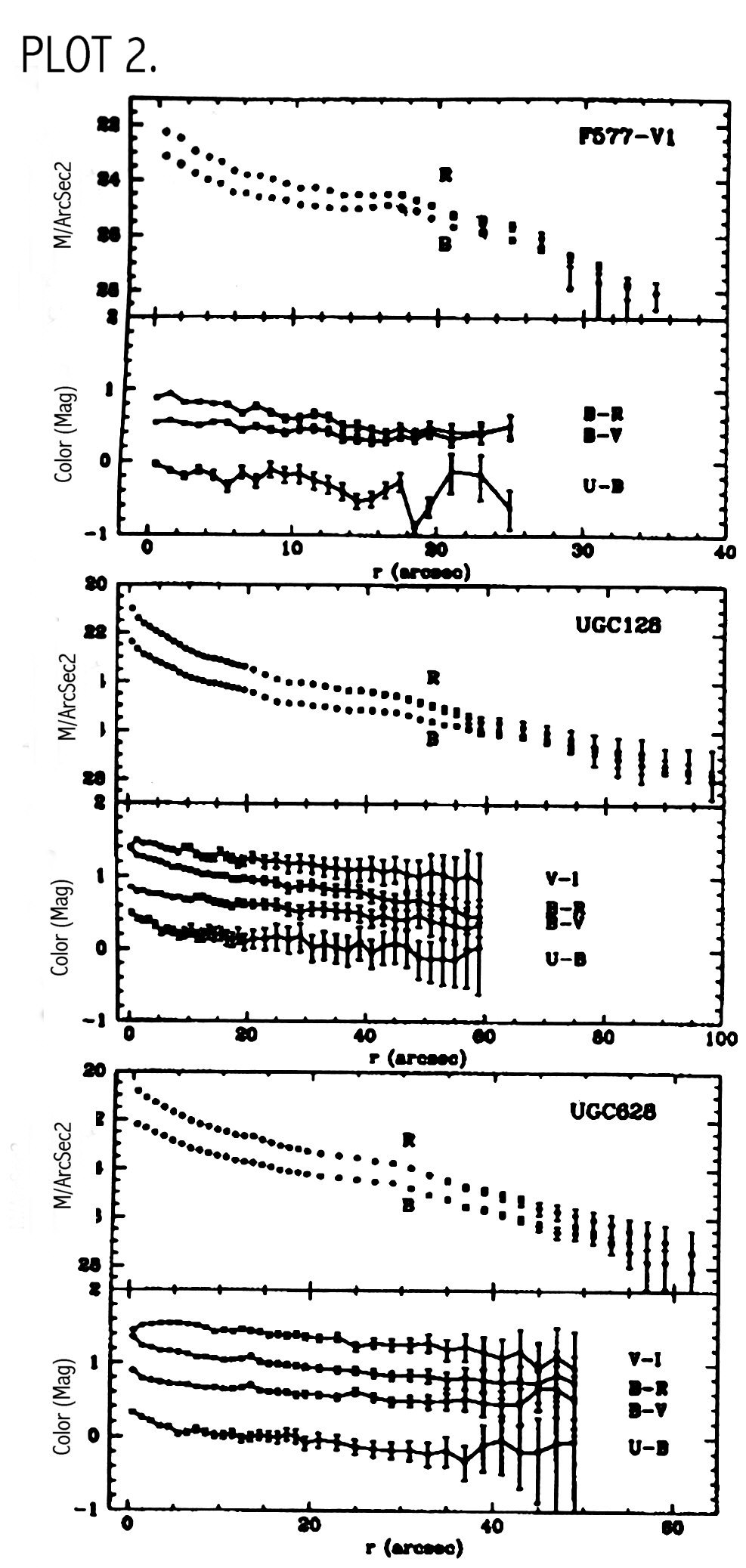
The B Magnitude is B=14.42 and the color is B-R=0.995. This corresponds well with values on the NED database. B-V = 0.597 and was obtained from the equation B-R= 1.5 (B-V) + 0.10. To make a plot of mag/arcsec2 vs distance along the major axis I used pvec to take a slice through the major axis. Pvec creates a plot file, which I called Bremnsky2.ma and Rremnsky2.ma. In pvec I used a position angle of 151 and a diameter is 1450. The width of the slice is 20 pixels. These files were then opened in IDL and plotted. Readout.pro reads in pvec major axis files with x in pixels and y in counts/pixel and converts to kpc and mag/arcsec2 and Lsun/pc2 using standard conversion procedures (see appendix A) (PLOT 1). Plot 2 shows brightness profiles for other LSB galaxies taken from de Blok, van der Hulst and Bothun (1994).o

The B-band image was used for the remainder of the calculations since the R-band image was very contaminated by the bright foreground star. The B-band image was converted to a face on surface brightness (in L_sun/pc²⁾ using an exponential disc to approximate the brightness profile in the procedure faceon.pro. The inner and outer regions of the brightness profile were approximated using a method from van der Kruit and Searle, 1980:
 

Face on: m (r)= u0 exp (-r/h) sech2 (z/z0)

Edge on: m(r,z)=m(0,0) [(r/h)K1(r/h)] sech2 (z/z0)

Where m (0,0)= 2 hL0 and K1is the modified Bessel function

Asymptotic solutions:

r/h<<1: [(r/h)K1 (r/h)]= 1+ r2/2 h2 ln (r/2 h)

r/h>>1: [(r/h)K1 (r/h)]= (pr/2 h) 0.5exp (-r/h)

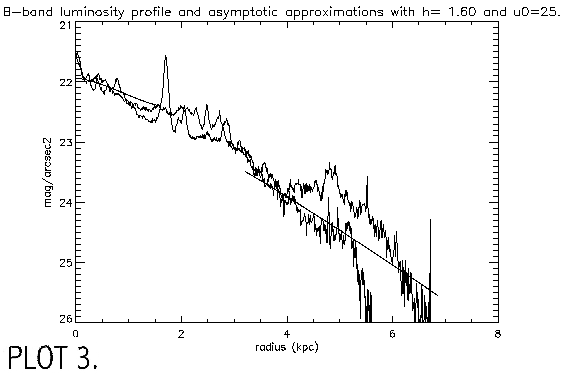
Here the value for z0 is 0.36 kpc and since I am looking along the major axis z=0, so the sech term equals 1. The best values were h=1.6 kpc and u0= 25 L_sun/pc². To derive an equation for the mass in stars, I first calculated to find the cumulative mass with increasing radius. Using a procedure called qromb in IDL I integrated over Lsun/pc2 *2p r to get the cumulative luminosity with radius. For mass I multiplied by the mass to light ratio. Then to get in form to be plotted on rotation curve, V² = GM/R,
 

Vstars2= G/R* M/L* ò S (Lum) 2p r dr

These two equations were substituted into the equation for the brightness profile and I ran the procedure many times, changing the values for h and u0, until a satisfactory fit was obtained (PLOT 3).

 
 

HI DATA

Lynn Matthews provided the HI 21-cm datacube of UGC 711 which was taken with the VLA in the BnC configuration. The beam size of the measurement is 24.55 arcsec (~1.2 kpc). The original data was read into AIPS with the task fitld. The data was cleaned 4000 times and saved as file UGC711.C4000. To derive a velocity profile I used two different methods: an intensity weighted mean (IWM) and gaussian fits to the line profile at positions along the major axis. For the gaussian method I first made a position velocity plot from the original datacube, using tvwin to cut out as much of the excess background that I could. The galaxy was then rotated to a vertical position (aparm(3)=60) using the task lgeom. This was done in preparation for the next step using xsum. I summed the x and y axis to make a 2d plot with axes velocity and declination, using the task xsum. This creates a plot of all the velocity components at a given radii and is called UGC711.C4000.POSVEL (PLOT 4).

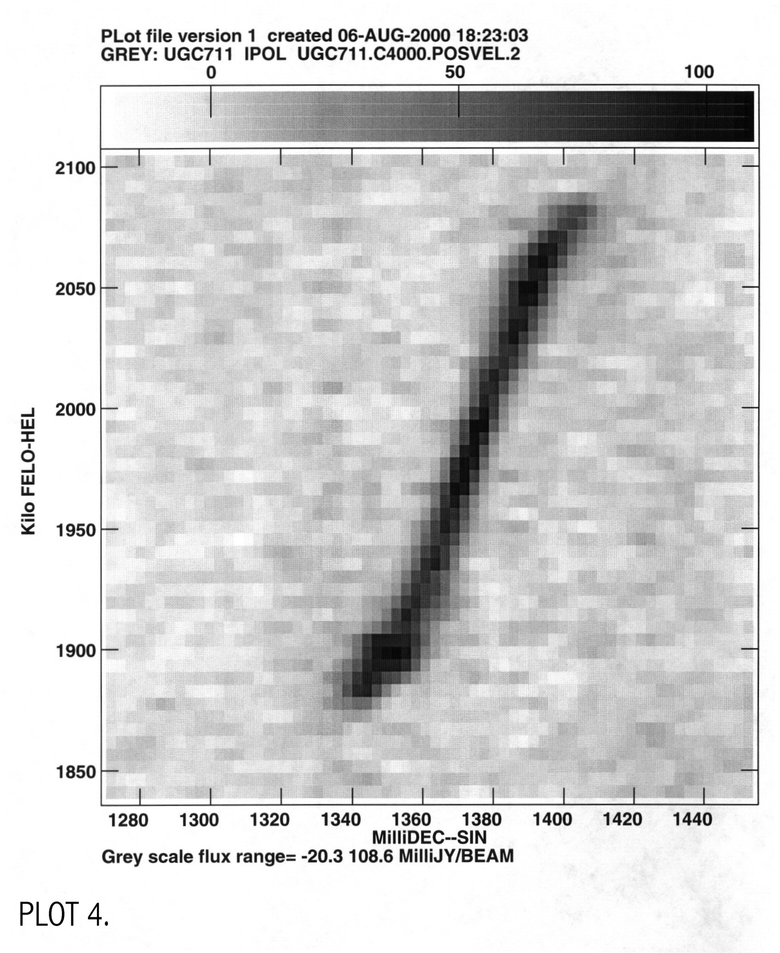
For a rotation curve only the radial velocity, which is the most Doppler shifted, is used. I used a procedure called xgaus to take vertical slices through the major axis at each pixel and fit a single gaussian to the peak velocity. This data, called UGC711.VEL (also created errors fwhm), was then plotted in IDL using a procedure called readgauss.pro which converts from m/s vs pixel to km/s vs kpc, using a distance to the galaxy of 10 Mpc. X zero and V zero were changed, and the velocity profile replotted until the left and right sides of the plot lined up. I also derived a velocity profile using a two gaussian fit, but the results were not as accurate. 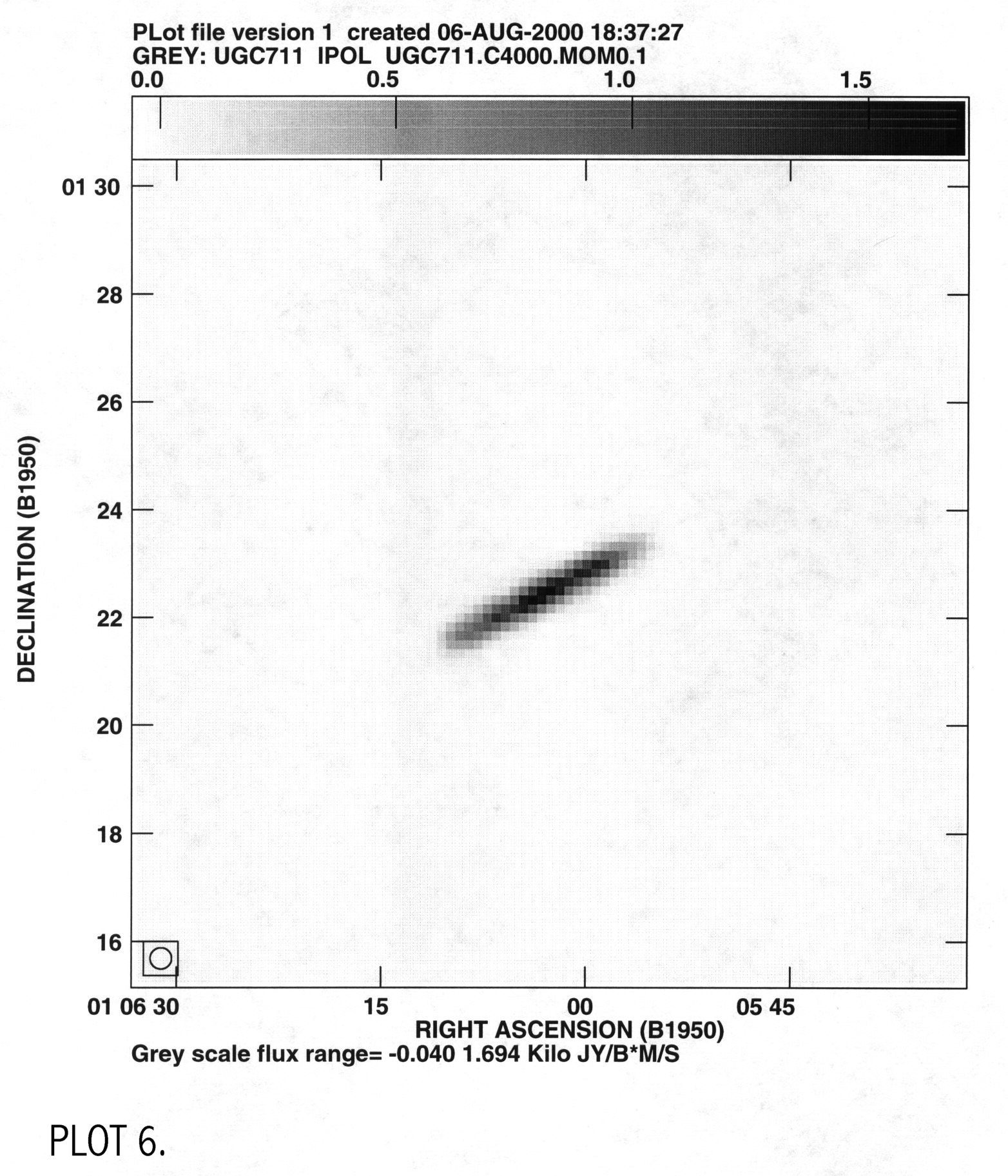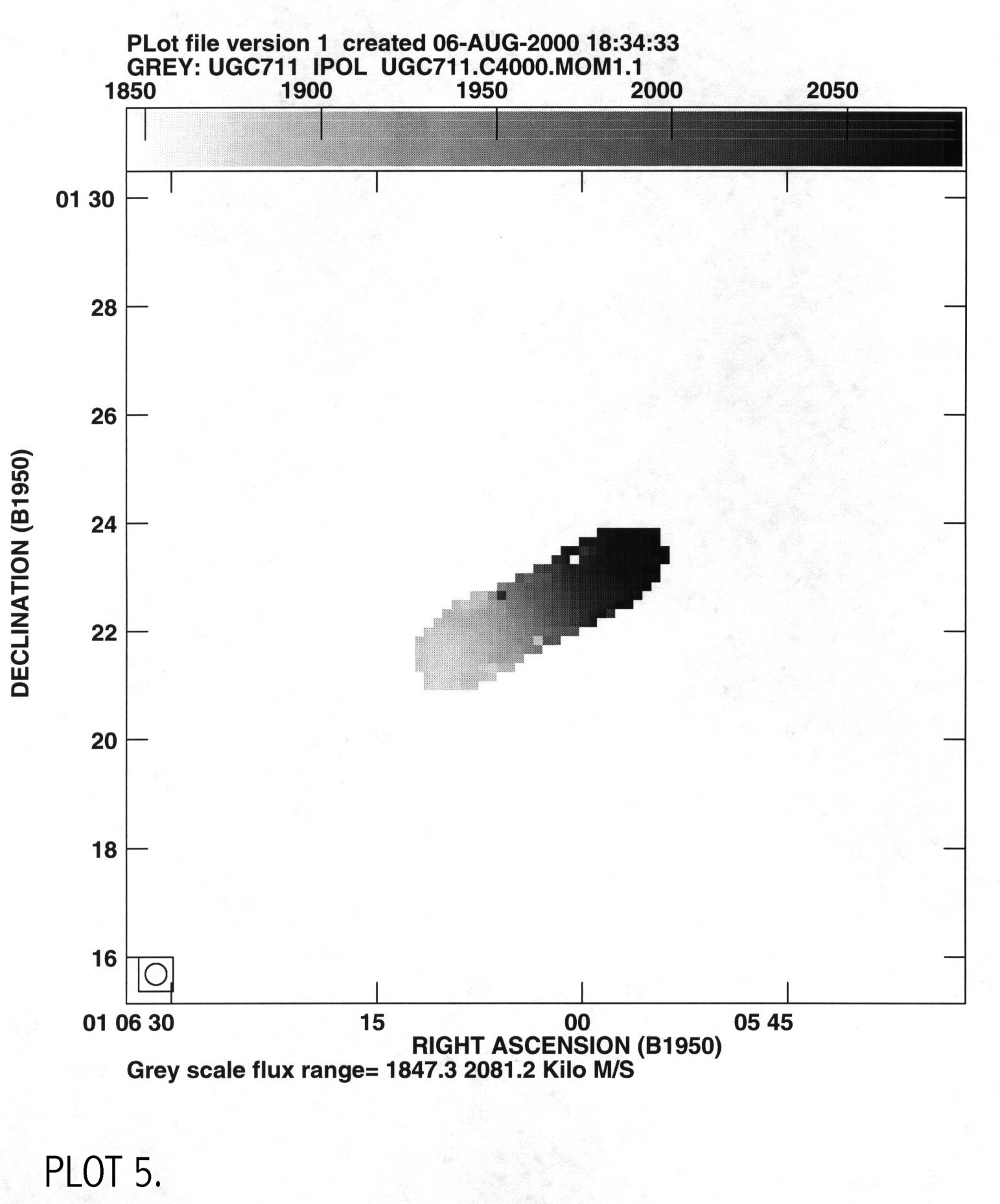As an alternate method to creating a rotation curve, I used an intensity weighted mean method after making moment maps. From the original data cubes I transposed the axis from LMV to VLM using trans (transcode= 312). Then using momnt I made moment 0,1,2 maps. This was done in an iterative way, slowly raising the value of the parameter icut excluding as much spurious signal as possible, without leaving out too much of the emission from the galaxy. Moment 1 gives a map of the intensity of the velocity at different radii and moment 0 gives a brightness map of the HI (PLOT 5 & 6). 
 
 

To get major axis profiles I used the tasks slice and sl2pl. I used slice to move these to a FITS directory where they are called UGC711.MOM1SLICE and UGC711.MOM0SLICE. These plots had units of m/s vs pixel and mJy/b km/s vs pixel, which were converted to km/s vs kpc and Msun/pc2 vs kpc, and plotted in IDL using a procedures named readmoment1.pro and readmoment0.pro. I then compared my two velocity profiles, the one from the gaussian fits and from moment 1 (PLOT 7).

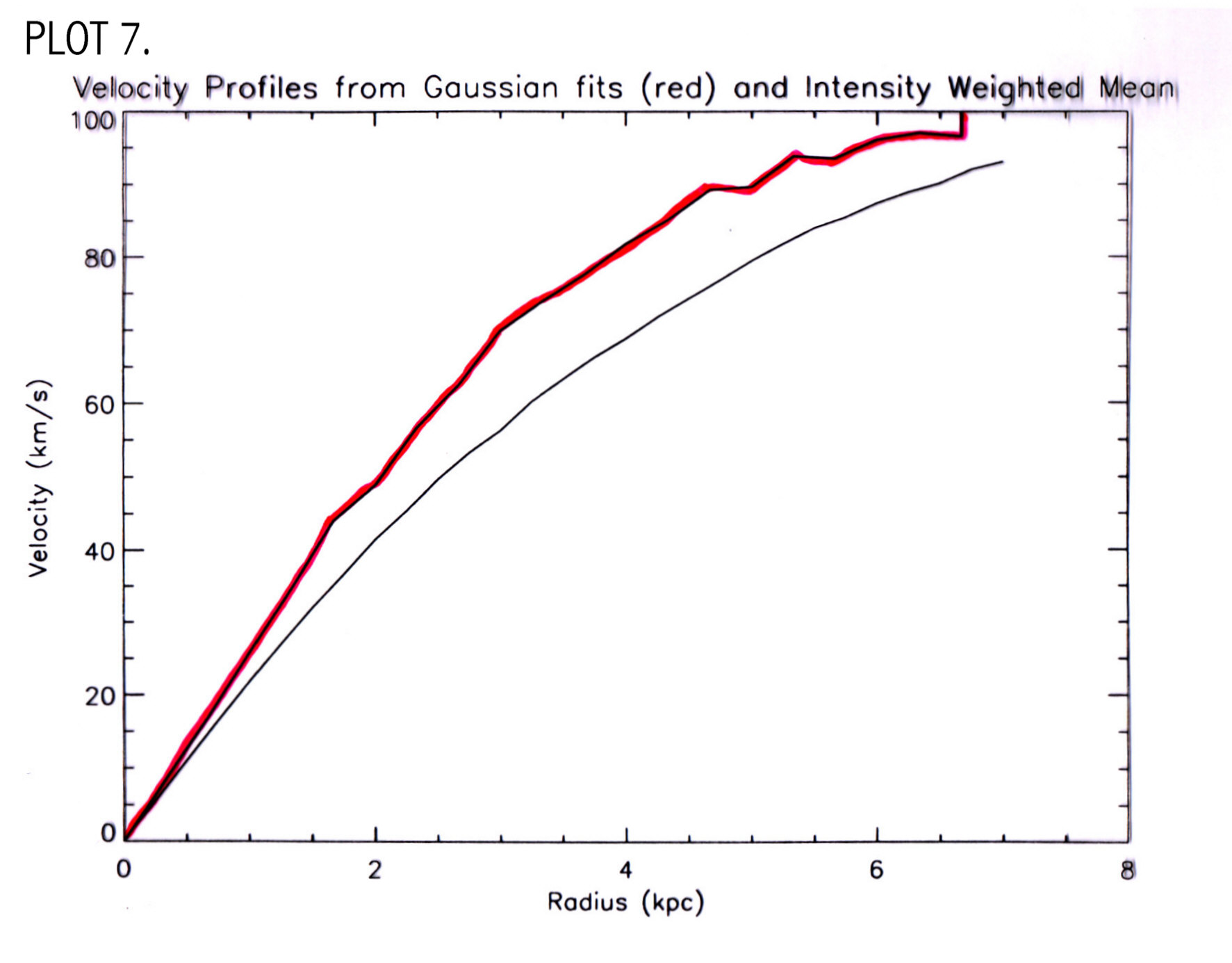
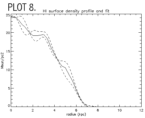
V zero for moment 1 is the same value determined from readgauss.pro; x zero and y zero were changed until the left and right sides of the velocity profile were aligned. This plot shows that the gaussian fit gives a more accurate plot of the radial velocity since the inner regions of this plot rise steeper than the IWM plot. The gaussian fits method fit a curve to the peak velocity while the IWM method can give a value offset from the peak. The plot rises to a velocity of 100 km/s, which is consistent with other LSB galaxies (Swaters, 1999), and infers a dynamical mass of M_dyn=3x10¹⁰ solar masses. Moment 0 is plotted to show the HI density profile of the galaxy, using the same zero values as determined from symmetrizing the moment 1 velocity curve (PLOT 8).

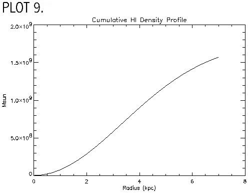
I converted this to a face-on profile using assuming a gaussian radial gas surface brightness distribution : A0*exp[ -(r-A1)²/(2*A2)]. Lynn Matthews gave the values for A0, A1, and A2 equaled to 1676.15, 0.28847, and 6.80364, respectively. I then integrated over this and multiplied by 2p r and the ratio of the total gas mass to the HI gas mass to get a cumulative mass for the gas. The total gas in the galaxy is M_gas=2x10⁹ solar masses which is reasonable according to the 1994 de Blok paper (PLOT 9). This is added to the rotation curve using an equation similar to that of the stars with a term to account for the contribution of He to the mass in gas:

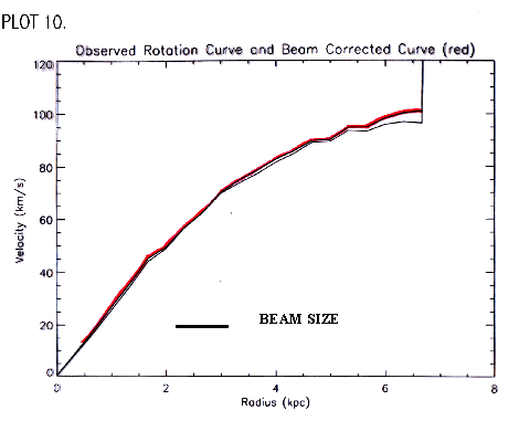
Before evaluating the rotation curve, beam smearing is taken into account. HI emission is smeared out due to the finite beam size of the telescope. This causes shallower gradients in the velocity field, which makes the inner part of the rotation curve less steep (Swaters, 1999). The inner part of the rotation curve is most affected by beam smearing; as this is where the curve is changing the most, you need more points to accurately connect them. To correct for beam smearing, a model curve was chosen and then a beam smear term was added to match the observed rotation curve. An arctan curve model was chosen of the form v(R)= (2/p) * v_c* arctan(R/rt), where vc is the maximum velocity and rt is the transition radius between the rising and the flat part of the rotation curve (S. Courteau, p 2408). This equation was then used in the beam smear correction equation of Kor Begeman pg. 40, 1987 (Equation 3) (See appendix B).

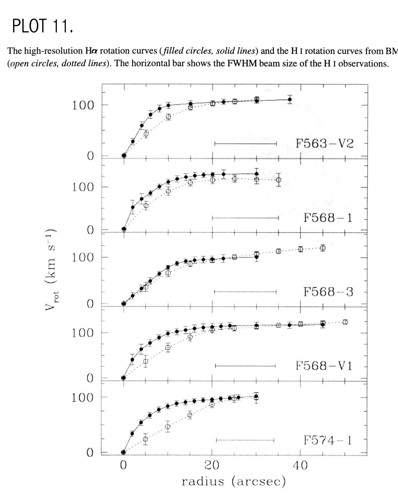
where v(x,y) is the arctan model, n(x,y) is the HI profile, ¶ N/¶ x is the partial derivative of the HI profile, and a is beam size (FWHM) divided by 2.35. Plot 10 shows the observed rotation curve and the beam corrected curve.The difference between the observed rotation curve and the beam corrected curve is very small. The small correction seems consistent with other LSB galaxies shown in PLOT 11 (Swaters, 1999). Here, even with a much larger beam size with only about 2 beams per radius, where UGC 711 has almost 7 beams per radius, the beam smear correction is very small. This makes sense for LSB galaxies since the inner regions of the curve for these galaxies rises slowly, due to the lack of a central bulge (Swaters, 1999).

 
 

The total rotation curve is expressed as the sum of the stellar, gas, and halo components.

The contribution from dark matter is calculated assuming an isothermal halo, which has the form

where r₀= central density in Msun/pc3 and r_c= core radius in kpc
To solve for these components and plot their contribution to the rotation curve I used a task in IDL called curvefit. One of the major uncertainties in fitting mass models to rotation curves is the uncertainty in the contribution of the stellar disk to the rotation curve. Lower and upper limits can be obtained by assuming that the contribution of the stellar disk is either minimal or maximal (Swaters, et al, 2000). Here I use curvefit to solve for the maximum disk mass to light ratio. Curvefit solved for the parameters r ₀, r_c, M/L, which is a prodecure written as calcV2.pro. The best fit to the observed rotation curve has values of r₀=0.05 Msun/pc3, r_c=2.9 kpc, and M/L=0.6 M_sun/L_sun. These values are compared with values for other LSB galaxies in PLOT 12. The value of central density is high; describing a dark matter dominated galaxy. The value for core radius is low compared with the other galaxies, consistent with a dark matter halo that dominates the mass of the galaxy (PLOT 12, from Swaters pg. 149, 1999).
 

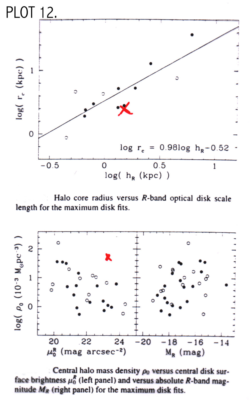
The M/L ratio is very low, especially since this is for a maximum disk situation. The value of M/L should be around 1.0 M_sun/L_sun, according to other galaxies with around the same B-R and B-V color index (U1230 from de Blok and McGaugh pg. 542, 1997). With a mass to light ratio of 0.6 M_sun/L_sun the mass contribution of the stars is 3.24x10⁸ solar masses. When the gas component was added to the equation, curvefit gave negative values for M/L, so the gas component is left out of the final rotation curve plot. 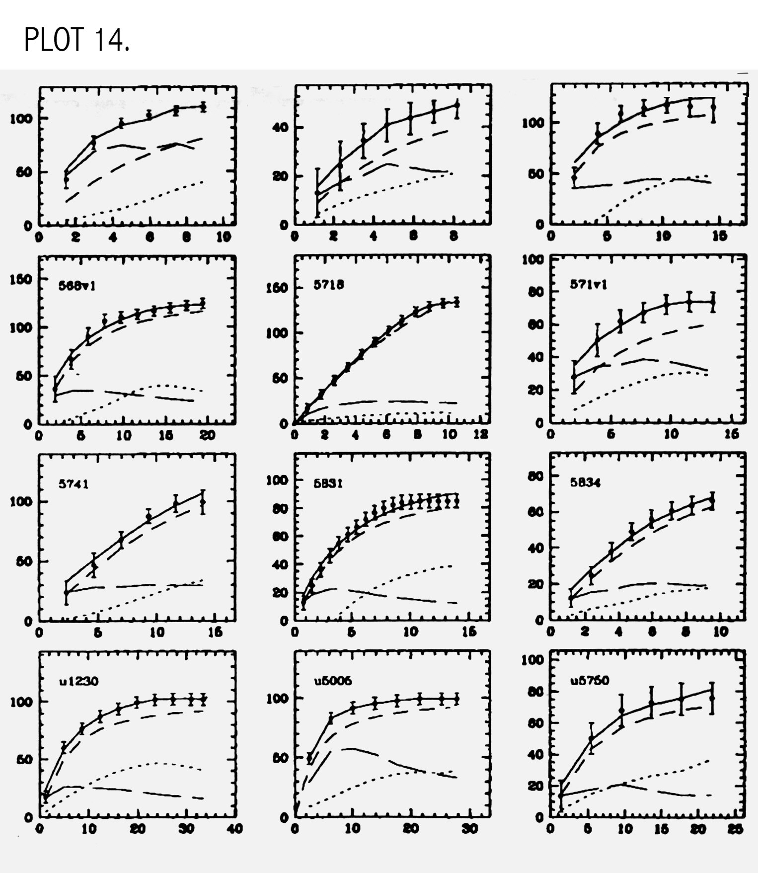Plots 13 show the observed rotation curve with stellar and halo components. When compared to other LSB rotation curves (PLOT 14), it is noted that the halo component makes up the majority of the rotation curve.
 

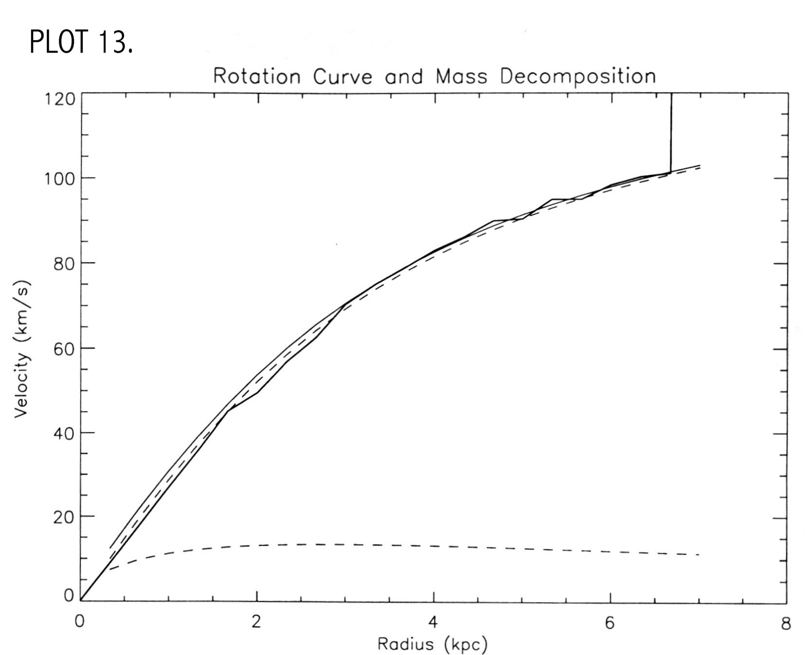
The lower slashed line is the contribution from the stars, the solid line that starts at the origin is the observed, beam corrected rotation curve, the other slashed line is the contribution from the halo and the other solid line is the sum of stellar and halo components. The dotted line is the contribution from the stars, the long slashed line is the contribution from the gas, the short slashed line is the contribution from the halo, and the solid line is the observed rotation curve. (From de Blok and McGaugh pg. 540, 1997).
 
 

Using an arctan model for the rotation curve gives a small correction for beam smearing; however the rotation curve derived for UGC 711 rises too slowly in the inner regions to accommodate a reasonable value for the mass to light ratio and for the addition of the gas component. A model rotation curve that rises more steeply in the inner regions, where the optical disk presumably dominates, may be more appropriate. Another possible source of error may lie in the dark matter halo model. Here I am using an isothermal halo model, where some alternate model may yield more accurate results. Had time allowed, I would have tried using another program for mass modeling in conjunction with the procedure curvefit in IDL, to solve for the stellar and halo parameters. The results do show, regardless of the errors, that this galaxy is almost completely dominated by dark matter, with a dark matter mass contribution of approximately M_dark=3.0x10¹⁰ solar masses.

Begeman, Kor. "HI Rotation Curves of Spiral Galaxies". Dutch Thesis 1987.

Broeils, Adrick. "Dark and Visible Matter in Spiral Galaxies". Dutch Thesis 1992.

Courteau, S. "Optical Rotation Curves"

De Blok, W.J.G, and S.S McGaugh. "The Dark and Visible Matter Content of Low Surface Brightness Disc Galaxies". 1997.

De Blok, W.J.G, J.M van der Hulst and G.D Bothun. "Surface Photometry of Low Surface Brightness Galaxies". 1994.

Matthews, L.D, J.S Gallagher III, and W. Van Driel. "The Extraordinary `Superthin' Spiral Galaxy UGC 7321. I. Disk Color Gradients and Global Properties from Multiwavelength Observations".
The Astronomical Journal, 1999 December.

Swaters, Rob. "Dark Matter in Late-Type Dwarf Galaxies". Dutch Thesis 1999.

Swaters, R.A., B.F Madore, and M. Trewhella. "High-Resolution Curves of Low Surface
Brightness Galaxies". The Astrophysical Journal, 2000 March 10.

Van der Kruit, P.C, and L. Searle. "Surface Photometry of Edge-On Spiral Galaxies I.
A Model for the Three-dimensional Distribution of Light in Galactic Disks". 1980.
 
 

Conversion from pvec major axis files with x in pixels and y in counts/pixel and converts to kpc and mag/arcsec2 and Lsun/pc2 using standard conversion procedures

Pixels to kpc

Pixels*10/60 * distance to galaxy in Mpc * 0.2909

D= 10 Mpc, multiply by 10/60 to get in arcmin, 0.2909 is conversion factor from arcmin to Mpc to kpc

Counts/pixel to mag/arcsec2

b= -2.5 log (counts/pixel for B-band)

Bmag (mag/arcsec2)= Equation 1 (using above b) + 26.0 + 5 log (0.195)

26.0 is zeropoint magnitude, 0.195 is arcsec/pixel for optical data

r = -2.5 log (counts/pixel for R-band)

(B-R)mag (mag)= Equation 2 (using above b-r)

Rmag (mag/arcsec2)= Bmag - (B-R)mag

Counts/pixel to Lsun/pc2

Blum= 10^[0.4 * (Bmag- 27.055)]

Rlum= 10^[0.4 * (Rmag- 25.885)]
 
 

Beam Smear Correction from Kor Begeman, 1987

N(x,y) is the projected neutral hydrogen distribution of a galaxy in the plane of the sky

v(x,y) is the velocity field of the galaxy, at rectangular coordinates x and y

n(x,y) is the amount of neutral hydrogen at position (x, y)

aand b are the beam corrections for x and y

V(x,y)= v(x,y) + 1/n(x,y) [(¶ v/¶ x * ¶ N/¶ x * a²) + (¶ v/¶ y * ¶ N/¶ y * b²)

+ N(x,y)/2n(x,y) [(¶²v/¶ x² * a² ) + (¶²v/¶ y² * b²)]

For my calculations only the x coordinate matters since the profile is along the major axis. So, all partial derivatives with respect to y drop out. v(x,y) is the arctan model, n(x,y) and N(x,y) are both the HI profile, and a is beam size/2.35 (Equation 3)