Next: Practical Applications of a Relational Database of FITS Keywords
Previous: Synthetic Images of the Solar Corona from Octree Representation of 3-D Electron Distributions
Up: Modeling
Table of Contents - Index - PS reprint

---

Astronomical Data Analysis Software and Systems VI
ASP Conference Series, Vol. 125, 1997
Editors: Gareth Hunt and H. E. Payne

---

Error and Bias in the STSDAS fitting Package

I. C. Busko
Space Telescope Science Institute, Baltimore, MD 21218, E-mail: busko@stsci.edu

Abstract:

1. Introduction

The two basic techniques used in the STSDAS fitting package are: (i) linear functions (Legendre and Chebyshev polynomials, cubic splines) are fitted by minimizing , solving the normal equations by the Cholesky method. Function coefficient errors are computed directly from the covariance matrix. This technique is provided by the IRAF (Image Reduction and Analysis Facility) library curfit. (ii) any function, linear or non-linear in its coefficients, can be fitted by minimizing using the downhill simplex method, also known as amoeba. This method is unable by design to compute coefficient errors. The package relies on an independent technique ( bootstrap resampling) to estimate these errors.

This work aims at assessing the reliability of coefficient estimates and error bars generated by both methods.

2. Method

Artificial data sets were generated from two functions: a 3rd degree power-series polynomial and a sum of two Planck functions. Each function was replicated 30 times and in each replication an independent noise realization was added at a fixed signal-to-noise level. Noise types included pure Gaussian, pure Poisson and a mixture of Gaussian plus Poisson. A separate, 30-element data set was created for each signal-to-noise level studied. Signal-to-noise spanned the range from ~1000 down to ~1 in logarithmic steps.

Each individual data set was fitted by the appropriate fitting task and results were output to tables. The power series polynomial was fitted by both linear and non-linear methods.

From the 30 measurements of each function coefficient , and its estimated error , i = 1, 2 ... 30, three statistics were computed:

• The average of coefficient error estimates
• The standard deviation of coefficient measurements
• The average ``residual'' coefficient (measured minus true)
  

If the coefficient computation is unbiased, should distribute itself around zero. If any bias is present, the average of the distribution will depart from zero. On the same grounds, if the coefficient error estimates are unbiased, that is, if they reflect the population true standard deviation, the difference should also distribute itself around zero.

 
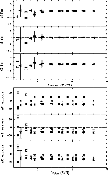
Figure: Power-series polynomial bias and errors. Ordinate is ``estimated - true'' coefficient residual (upper panel) and error bar (lower panel), in a relative (percent) scale, for the three first lower-order polynomial coefficients. Abscissa is signal-to-noise. Each point depicts the average of 30 measures; error bar depicts the standard deviation of the same 30 measures. Solid symbols: non-linear algorithm. Open symbols: linear algorithm. Squares: Poisson noise. Triangles: Gaussian noise. Points below the zero line mean that the coefficient (or its error) is systematically underestimated; above the line it is overestimated. Original Postscript figures(112kB), (64kB).

 
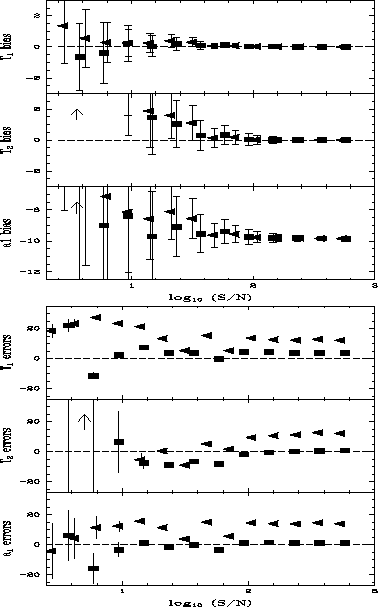
Figure: Double Planck function bias and errors. The two temperatures and the largest black-body amplitude are depicted. See caption for Figure 1. Original Postscript figures(128kB), (136kB).

3. Results

Results are summarized in the Figures.

When applied to a power-series polynomial with Gaussian noise, both linear and non-linear techniques generated unbiased coefficients at the level of <1% for any tested S/N ratio. Poisson noise introduced underestimation bias at a level of a few percent for lower (~2-5) S/N data. The largest bias was seen on polynomial's zero-order term, induced perhaps by the non-symmetric nature of the Poisson distribution. A different behavior was seen when fitting the strongly non-linear sum of two Planck functions. The dominant (in intensity) black-body had its temperature determined with almost no bias down to S/N ~ 2. The weaker component, however, showed significant overestimation bias at low S/N. The dominant black-body's amplitude showed large (~8-10%) underestimation bias, and the weaker amplitude did not give significant results. This can be interpreted as the result of both amplitudes being confused into a single one by the fitting algorithm, thus resulting in a biased estimate for one of them. The noise model seems to play no role in these results.

When fitted by the non-linear algorithm, the power-series polynomial errors showed a systematic underestimation of ~10-20 percent, seemingly independent of noise type. The linear algorithm, on the other hand, delivers errors which are off from the ``true'' ones by amounts that depend on noise type, and might also depend on the coefficient values themselves. The double black-body function fit showed errors that lie close to the true ones in the Gaussian noise case, and with systematic overestimation of ~20 percent in the Poisson noise case.

As a general rule one might say that bias at a few percent level should be expected when fitting either non-linear functions, or linear functions with Poisson noise, in particular with low S/N data. Also, error bars generated by both linear and non-linear methods are prone to under or overestimate the ``true'' errors by as much as 10-20 percent, even with high S/N data. The details, though, seem to be dependent on the functional form and noise type.

Next: Practical Applications of a Relational Database of FITS Keywords
Previous: Synthetic Images of the Solar Corona from Octree Representation of 3-D Electron Distributions
Up: Modeling
Table of Contents - Index - PS reprint