3.7 Model integration

The principal steps in calculating the brightness distributions are as follows:

1. Construct grids to match the observations at each of the two resolutions.
2. At each grid point, determine whether the line of sight passes through the jet. If so, calculate the integration limits corresponding to the outer surface of the jet and, if relevant, the spine/shear-layer interface. Separate ranges of integration are required to avoid discontinuities in the integrand.
3. Integrate to get the Stokes parameters I, Q and $U$ using Romberg integration. The steps needed to determine the integrand are outlined below.
4. Add in the core as a point source.
5. Convolve with a Gaussian beam to match the resolution of the observations.
6. Evaluate $\chi ^2$ over defined areas, using an estimate of the ``noise level'' derived as described later.

In order to determine the I, Q and U emissivities at a point on the line we follow an approach described in detail in Laing 2002 and based on that of Matthews & Scheuer (1990). We neglect synchrotron losses, on the grounds that the observed spectrum is a power law with $\alpha = 0.55$ between 1.4 and 8.4 GHz (and extends to much higher frequencies; Hardcastle et al. 2002). The emissivity function $\epsilon \propto n_0 B^{1+\alpha}$, where B  is the total field and n₀ is the normalizing constant in the electron energy distribution as defined in Section 3.1. The observed emissivity can be calculated in the formalism developed by Laing (2002) by considering an element of fluid which was initially a cube containing isotropic field, but which has been deformed into a cuboid by stretching along the three coordinate directions by amounts proportional to the field component ratios in such a way that the value of $\epsilon$ is preserved. We calculate the synchrotron emission along the line of sight in the fluid rest frame, thus taking account of aberration.

The main steps in the calculation are:

1. Determine coordinates in a frame fixed in the jet, in particular the radial coordinate $\rho$ and the streamline index $s$, numerically if necessary.
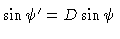
2. Evaluate the velocity at that point, together with the components of unit vectors along the streamline coordinate directions (and hence the angle between the flow direction and the line of sight $\psi$). Derive the Doppler factor $D = [\Gamma (1 - \beta\cos \psi)]^{-1}$ and hence the rotation due to aberration ( $\sin\psi^\prime = D\sin\psi$, where $\psi^\prime$ is measured in the rest frame of the jet material). Rotate the unit vectors by $\psi - \psi^\prime$ and compute their direction cosines in observed coordinates.
3. Evaluate the emissivity function $\epsilon$ and the rms components of the magnetic field along the streamline coordinate directions (normalized by the total field). Scale the direction cosines derived in the previous step by the corresponding field components, which are $j/(1+j^2+k^2)^{1/2}$ (radial), $1/(1+j^2+k^2)^{1/2}$ (toroidal) and $k/(1+j^2+k^2)^{1/2}$ (longitudinal) in the notation of the previous section.
4. Evaluate the position angle of polarization, and the rms field components along the major and minor axes of the probability density function of the field projected on the plane of the sky (Laing 2002). Multiply by $\epsilon(\rho,s)D^{2+\alpha}$, to scale the emissivity and account for Doppler beaming.
5. Derive the total and polarized emissivities using the expressions given by Laing 2002 and convert to observed Stokes Q and $U$.

2002-06-13