Figure 1
Last changed November 28 1997
"Lab notebook" web page of Darrel Emerson(http://www.tuc.nrao.edu/~demerson/magnet.magnet.html)
These tests describe measurements made on several fluxgate magnetometer
sensors made by Speake & Co., supplied in the USA by
Fat Quarters
Software and Electronics. More information may be obtained
from Erich Kern. I have no personal
connection with either company. The magnetometers are particularly
sensitive, and are designed to measure small fluctuations in the
geomagnetic field. The model FGM-3h is the most sensitive in
the range of sensors available from Fat Quarters Software, and in
fact is so sensitive that it will saturate if aligned N-S along
the Earth's field. It is normally used aligned in the E-W direction,
which is equivalent to measuring the "Y" term of the field; this
is approximately proportional to the magnetic declination D.
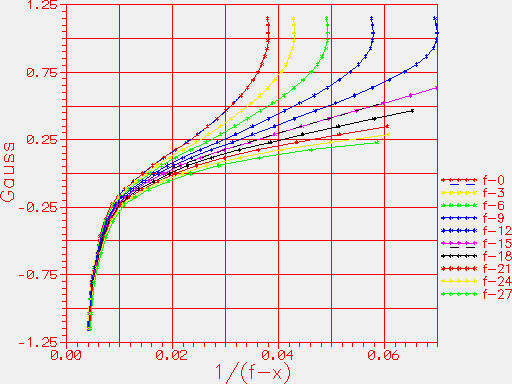
Here are some test measurments on the first FGM-3h fluxgate magnetometer received from Fat Quarters Software. The magnetometer zero field was found to correspond to a frequency of close to 68 kHz. This was found:
(1) by setting the magnetometer as close as possible to the magnetic E-W axis, and (2) by finding the alignment of the magnetometer such that, when it was reversed end-to-end, the output frequency remained the same.
Figure 1
The vertical axis gives the magnetic field surrounding the magnetometer. This was calculated from the current through a solenoid into which the magnetometer was placed. The solenoid was about 3 times longer than the magnetometer, with the FGM-3h placed in the centre of the solenoid. The solenoid length/diameter ratio is about 6.64:1. Before making the measurements, the solenoid and magnetometer were aligned along a magnetic E-W axis, to minimize the effect of the Earth's field.
The horizontal axis is derived from the frequency of pulses from the magnetometer. The frequency was measured with a counter. From the frequency, the quantity (1/(F-x) ) is calculated, with F the frequency in kHz, and x an offset. Offset values for x of 0,3,6,9,12,15,18,21,24 and 27 were used. Ten plots are shown, corresponding to the same data, but with different "x" values used to calculate the horizontal coordinate on the graph.
Note however that none of the curves give a linear response centered on the zero-field measurement. The response does not start becoming even vaguely linear until positive magnetic fields are applied. Note that the zero-field pulse frequency of 68 kHz corresponds to 0.0147 along the X-axis for the "x=0" curve, or 0.019 on the "x=15" curve (i.e. 1/(F-15)).
Note that the plot against (1/(F-15)) gives a reasonably linear response from solenoid. The solenoid length/diameter ratio is about 6.64:1. Before making the measurements, the solenoid and magnetometer were aligned along a magnetic E-W axis, to minimize the effect of the Earth's field.
The horizontal axis is derived from the frequency of pulses from the magnetometer. The frequency was measured with a counter. From the frequency, the quantity (1/(F-x) ) is calculated, with F the frequency in kHz, and x an offset. Offset values for x of 0,3,6,9,12,15,18,21,24 and 27 were used. Ten plots are shown, corresponding to the same data, but with different "x" values used to calculate the horizontal coordinate on the graph. The horizontal units have the dimension of milliseconds.
Note however that none of the curves give a linear response centered on the zero-field measurement. The response does not start becoming even vaguely linear until positive magnetic fields are applied. Note that the zero-field pulse frequency of 68 kHz corresponds to 0.0147 along the X-axis for the "x=0" curve, or 0.019 on the "x=15" curve (i.e. 1/(F-15)).
Note that the plot against (1/(F-15)) gives a reasonably linear response from about +0.2 gauss to at least +0.6 gauss or beyond.
Comparative measurements were made, using the original sensor measured above in October (sensor #1) and the two newer sensors (#2 and #3) on loan from Erich Kern. The new sensors are both FGM-3h types, but differ from #1 in (1) having pins rather than wires for the electrical connections and (2) having 4 pins. The extra pin is for an internal calibration or bias solenoid. The DC resistance from this extra pin to ground was measured at 9.0 ohms.
The measurements described below have not made use of this extra pin. The first measurement made was to determine the frequency corresponding to zero field. To do this, each sensor was experimentally aligned on a horizontal wooden table, approximately E-W, such that when the sensor was rotated through 180 degrees (E-W becoming W-E) the sensor frequency remained the same. There are some assumptions built into this way of finding the zero-field frequency, but it's probably pretty close to the right answer. The original sensor, #1, gave a frequency of 68.7 kHz. Sensor #2 gave 60.9 kHz, and #3 gave 62.0 kHz. These numbers are +/-0.5 kHz.
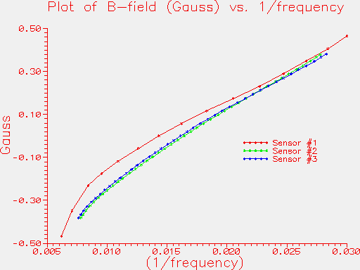
Figure 2
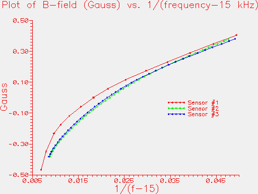
Figure 3
Conclusion: All three sensors are very similar. Looking at Figure 2, it is clear that the calibration of sensor #1 is significantly different from that of #2 and #3. The linearity at fields close to zero is better on sensors #2 and #3, as can be seen in both Figures 2 and 3. However, all sensors show greatest linearity for positive fields, say around +0.2 gauss. Although the calibration between #1, and #2 or #3, does appear to be somewhat different, it is not dramatically different.
A third batch of sensors were received, on loan from Erich Kern. Similar tests were performed. The results are summarised in the plot below, Figure 4, which includes the measurements of all 3 batches of sensors.
| Summary of sensors tested | |
|---|---|
| Sensor #1 | Original FGM-3h, with 3 wire leads |
| Sensors #2, #3 | Second batch, October 1997. 4 pin connections. |
| Sensors #4. #5 | Third batch, November 1997. 4 pin connections. |
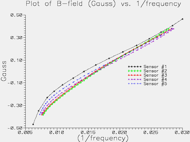
Figure 4
Figure 4 shows the comparison of all three batches of FGM-3h sensors. Horizontal axis is reciprocal frequency (kHz), so has units of milliseconds. The most recent batch, sensors #4 and #5, seem to be more or less intermediate in response between the original sensor #1 and sensors #2 and #3. There are no dramatic differences between any of the sensors.
In the above plots, the inverse of the slope of each line is an indication of relative sensitivity, in terms of a the period change which corresponds to a given change in magnetic field.
Figure 4 above shows that over a small range of field, say +/-0.1 Gauss, the response of (change in magnetic field) against (change in sensor signal period) is reasonably linear. The table below shows the results from fitting straight lines to the plots in Figure 4, only using the data between +0.1 to -0.1 Gauss.
| Sensor # | Batch | Change in field/Change in period, Gauss/millisecond | Hz/gamma at 60 kHz |
|---|---|---|---|
| 1 | I | 31.6 | 1.14 |
| 2 | II | 35.95 | 1.00 |
| 3 | II | 35.45 | 1.02 |
| 4 | III | 30.91 | 1.16 |
| 5 | III | 29.95 | 1.20 |
The slope of the fitted straight lines (column 3 in the above table) gives the change of field, in Gauss, required to change the period of the pulse stream from the magnetometers by 1 millisecond. Simple calculus enables this to be expressed in terms of Hz/gamma (1 gamma = 1 nT = 10-5 Gauss). Because the sensor is close to linear in period, not frequency, this sensitivity constant (Hz/gamma) depends on the applied magnetic field, or specifically varies as the square of the sensor's pulse frequency. To make useful comparisons, the sensitivity in Hz/gamma has been calculated assuming a sensor pulse frequency of 60 kHz, which corresponds to nearly zero field for all the sensors and is near the middle of their working range.
The above table shows that sensors of a given batch (#1=batch I, #2 & #3 = batch II, #4 & #5 = batch III) have comparable sensitivity, within about 3% of each other, but that batch 3 is approximately 17% more sensitive than batch 2. With the small number of samples, this is probably over-interpreting the data, but it is interesting to note.
The conclusion is that all sensors are relatively similar, although
there do seem to be small systematic differences between the batches. In terms
of sensitivity expressed as Hz/gamma, on the face of it the most
recent batch is, by a small
margin, the best.
My home is about 10 miles from the
Tucson Magnetic Observatory, one
of the official USGS observatories. Data from that observatory has just
kindly been made available to me. The plot below (Figure 5) shows a comparison
of my own data with that from the Tucson Magnetic Observatory for UT date
November 5th. This was a geomagnetically unsettled day.
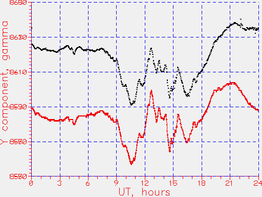
Figure 5. Superposed plots. Total vertical range 100 nT, with dashed horizontal lines every 20 nT
The upper (black) plot shows my own data, sampled nearly every 2 minutes, for
UT 0h - 24h on UT date 5th November 1997. My sensor is nearly E-W,
so is sampling the Y component of magnetic field. The Tucson Observatory
data were supplied as HDZF data, but the D value, in arc min, has been
converted to the conventional Y component, using the standard formula
(Y=H*sin(D)).
The lower (red) plot shows the data from the Tucson Magnetic Observatory,
sampled every minute.
The total range of the plot is 100 nanoTesla (nT), with grid lines drawn
every 20 nT. There is an arbitrary DC offset applied to the plots, to
be able to put them on to the same graph. When the above plots were made,
my convention of sign of the field was reversed; the two traces are
matched, but both are inverted with respect to usual practice.
As can be seen, there is excellent agreement between the data sets.
The Tucson Magnetic Observatory is about 10 miles from my home, so the
earth's magnetic field in the two locations should be nearly identical.
My own data (the upper plot) were calibrated with a home-made solenoid,
putting a known current through the coil. It seems as if my calibration
may be a few percent low, but I find the agreement quite remarkable.
The only significant difference is in the last 4 or 5 hours of the
UT day. The Tucson Observatory data show a gradual decline in field,
ending up at 24h very close to the value measured at 0h. My own data
stay more constant, ending up about 10 nT higher in measured field at
24h, compared to the 0h measurement. My guess is that this is a temperature
effect. Although I have tried to stabilize the temperature of my sensor
as far as feasible, there is bound to be some residual effect.
All in all, I'm delighted with this comparison.
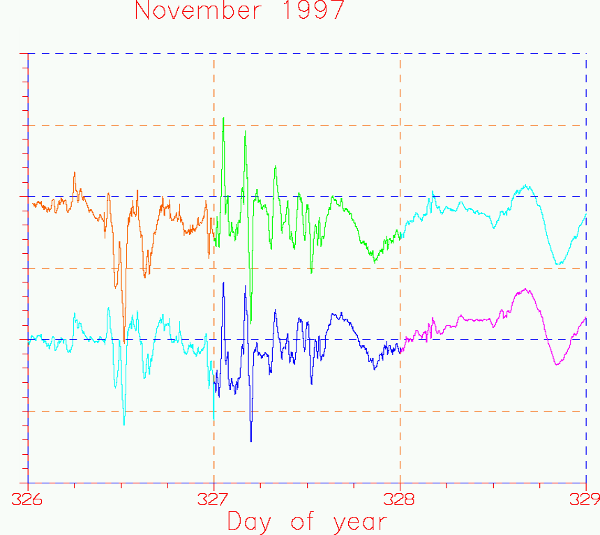
Below is a similar comparison between my own measurements of the Y-component
of the earth's field and the Tucson Magnetic Observatory's data. This
is a 3-day period from Nov 22 to Nov 24 UT date. The X-axis shows
day-of-year (from 0h UT on UT day 326, to 0h UT on day 329).
The vertical scale covers a total range of 300 gamma,
with horizontal dashed lines every 50 gamma. The sign convention
of field now follows normal practice, unlike Figure 5 above.
Figure 6. Superposed plots, covering 3 days of data. Total
vertical scale 300 nT, with horizontal dashed lines every 50 nT.
The upper trace shows the data from the Tucson Magnetic Observatory, while
the lower trace shows my own measurements with the FGM-3h sensor. (An arbitrary
DC offset has been applied to be able to show the two traces on the
same plot without confusion). The Tucson Magnetic Observatory data were
sampled every minute, but my data were only sampled about once every
2 minutes. Each day's data is shown in a different
color. Again, there is outstanding agreement between the two data sets.
The first two days (326-327) show magnetic storm conditions, which have
died down to reveal the normal quiet field diurnal variation
for about the last 10 hours of
day 328. Close
inspection does reveal some minor differences, but I do not know if these
are real differences (I am about 10 miles from the Tucson Magnetic Observatory,
and the physical alignment of my sensor is probably a few degrees different
from the true E-W of the Y component of field), or small drifts in the
sensor's output. The measurements track each other within about 10 nT,
which I find quite remarkable; even changes as small as 1 nT generally
correspond in the two datasets.