GPU Benchmarking

(8/29/2007) This page describes some early investiagtions into the use of GPUs for real time signal processing. Here I compare the performance of the GPU and CPU for doing FFTs, and make a rough estimate of the performance of this system for coherent dedispersion.

Hardware

CPU: Intel Core 2 Quad, 2.4GHz
GPU: NVIDIA GeForce 8800 GTX

Software

CPU: FFTW
GPU: NVIDIA's CUDA and CUFFT library.

Method

For each FFT length tested:

8M random complex floats are generated (64MB total size).
The data is transferred to the GPU (if necessary).
The data is split into 8M/fft_len chunks, and each is FFT'd (using a single FFTW/CUFFT "batch mode" call).
The FFT results are transferred back from the GPU.

The real time taken by each step is measured. The process is iterated and the times are averaged. All FFTs are done in-place. FFTW plans were computed with FFTW_MEASURE, and were not multi-threaded.

Results

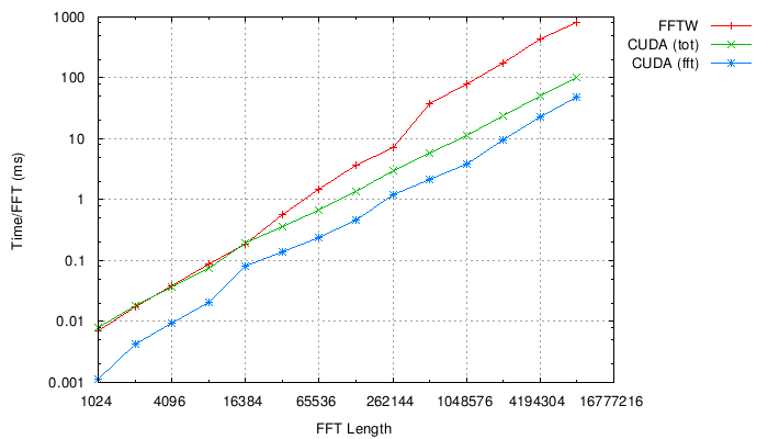
The first plot shows time taken per FFT. The CUDA results are shown with data transfer time included (CUDA(tot) line) or not (CUDA(fft) line). The GPU results here are seen to be dominated by the data transfer time:

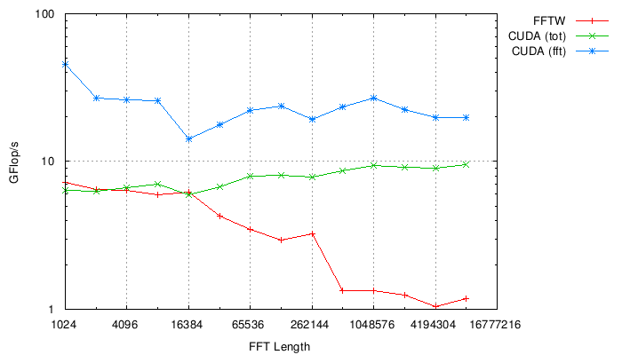
The same data plotted using FFTW's performance metric in Gflops:

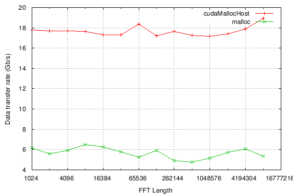
Finally, we can measure the data tranfer rate to/from the GPU for each trial. Performance is improved by allocating the transfer buffer using cudaMallocHost rather than plain malloc. The theoretical maximum data rate through a PCIe x16 slot is 31.25 Gb/s.

Coherent Dedispersion

We can use the numbers just measured to make a rough estimate of the total bandwidth that could be coherently dedispersed in real time by one of these systems. This estimate makes the following assumptions:

"ASP-like" system parameters: 4-MHz channels, 8-bit sampling.
Data unpacking (byte-to-float conversion) will be done in the GPU (reduces data transfer time per block by a factor of 4).
Detection and folding will be implemented in the GPU, so there will be only one significant data transfer and two FFTs per block.
The time needed for unpacking, filter multiplication, detection and folding is constant as a function of DM (or FFT length), and is set so that it is 25% of the total time at 32k FFT lengths. This is based on ASP experience, but could be totally wrong here! We won't know until the whole algorithm is tried in the GPU (Update: See below).
Overlap is 25% (or, FFT length is 4 times chirp length).
The data acquisition (from network, hard drive, EDT card, etc) can be done concurrently with dedispersion and does not negatively affect the PCIe transfer rate. This seems likely at these data rates, but hasn't been tested yet.

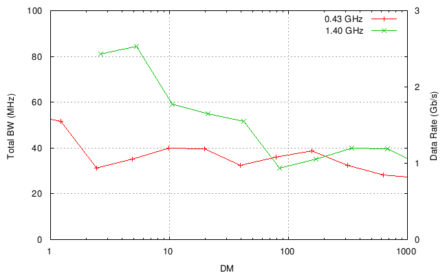
Given these assumptions, this plot shows the estimated total bandwidth that could be handled by one system, as a function of DM, for RFs of 430 MHz and 1.4 GHz:

Coherent Dedispersion, part II

(9/11/2007) This is a update on the possibility of performing coherent dedispersion on the GPU, after implementing and benchmarking a basic program to do so. The program performs the following steps, each of which is timed:

Approx. 25 MB of raw (8-bit, 2 pol, complex) data is transferred from main memory to the GPU.
The data are split into N_fft buffers, which are overlapped in time by one chirp length.
The 8-bit data is converted to single precision floating point.
Each buffer is FFT'd, multiplied by a chirp function, then inverse FFT'd.
The data are squared to form power and polarization cross products.
The results are then transferred back to main memory.

The program was run for chirp lengths ranging from 16 to 32k samples. For each chirp, FFT lengths from 2*(chirp length) to 4M samples were timed, and the best-performing FFT length was used to make the following plots. First, we can show the maximum real-time bandwidth as a function of chirp length. This also shows DM as a function of chirp length for several standard RF and channel BW combinations:

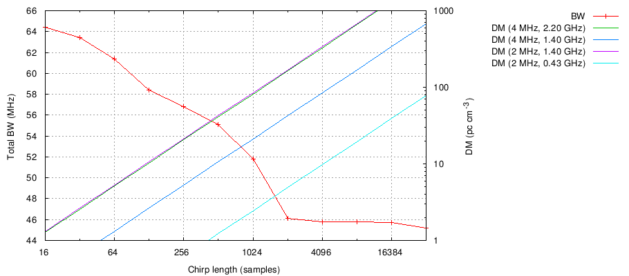
These results agree fairly well with the rough estimate of the previous section, especially in the high-DM regime where the FFT dominates the computation. More insight can be gained by looking at the timing breakdown for each of these trials. In all cases, the computation is dominated by three of the steps listed above: FFT (step 4, not counting the multiply), data transfer to/from GPU (steps 1 and 6), and overlapping the data (step 2):

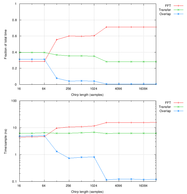
The data transfer time is constant, as expected. However, the overlap takes a significant amount of time at short chirps (many small FFTs), accounting for some of the discrepancy between these results and the rough estimate. This could potentially be improved by additional optimization of the overlap procedure (currently implemented using cudaMemcpy).

This test has addressed several of the assumptions of the previous section, with the exception of:

Data acquistion (no 10 GbE card to test this with yet).
Folding is not performed (see discussion below).