The continuous Fourier transform is important in mathematics, engineering, and the physical sciences. Its counterpart for discretely sampled functions is the discrete Fourier transform (DFT), which is normally computed using the so-called fast Fourier transform (FFT). The DFT has revolutionized modern society, as it is ubiquitous in digital electronics and signal processing. Radio astronomers are particularly avid users of Fourier transforms because Fourier transforms are key components in data processing (e.g., periodicity searches) and instruments (e.g., antennas, receivers, spectrometers), and they are the cornerstones of interferometry and aperture synthesis. Useful references include Bracewell [15] (which is on the shelves of most radio astronomers) and the Wikipedia¹¹ 1 http://en.wikipedia.org/wiki/Fourier_transform. and Mathworld²² 2 http://mathworld.wolfram.com/FourierTransform.html. entries for the Fourier transform.

The Fourier transform is a reversible, linear transform with many important properties. Any complex function $f(x)$ of the real variable $x$ that is both integrable and contains only finite discontinuities has a complex Fourier transform $F(s)$ of the real variable $s$, where the product of $x$ and $s$ is dimensionless and unity. For example, the Fourier transform of the waveform $f(t)$ expressed as a time-domain signal is the spectrum $F(\nu )$ expressed as a frequency-domain signal. If $t$ is given in seconds of time, $\nu$ is in ${\mathrm{s}}^{-1}=\mathrm{Hz}$.

The Fourier transform of $f(x)$ is defined by

$$\boxed{F(s)\equiv {\int }_{-\mathrm{\infty }}^{\mathrm{\infty }}f(x)e^{-2\pi isx}dx,}$$

(A.1)

which is usually known as the forward transform, and

$$\boxed{f(x)\equiv {\int }_{-\mathrm{\infty }}^{\mathrm{\infty }}F(s)e^{2\pi isx}ds,}$$

(A.2)

which is the inverse transform. In both cases, $i\equiv \sqrt{-1}$. Alternative definitions of the Fourier transform are based on angular frequency $\omega \equiv 2\pi \nu$, have different normalizations, or the opposite sign convention in the complex exponential. Successive forward and reverse transforms return the original function, so the Fourier transform is cyclic and reversible. The symmetric symbol $\iff$ is often used to mean “is the Fourier transform of”; e.g., $F(s)\iff f(x)$.

The complex exponential (Appendix B.3) is the heart of the transform. A complex exponential is simply a complex number where both the real and imaginary parts are sinusoids. The exact relation is called Euler’s formula

$$\boxed{e^{i\varphi }=\cos \varphi +i\sin \varphi ,}$$

(A.3)

which leads to the famous (and beautiful) identity $e^{i\pi }+1=0$ that relates five of the most important numbers in mathematics. Complex exponentials are much easier to manipulate than trigonometric functions, and they provide a compact notation for dealing with sinusoids of arbitrary phase, which form the basis of the Fourier transform.

Complex exponentials (or sines and cosines) are periodic functions, and the set of complex exponentials is complete and orthogonal. Thus the Fourier transform can represent any piecewise continuous function and minimizes the least-square error between the function and its representation. There exist other complete and orthogonal sets of periodic functions; for example, Walsh functions³³ 3 http://en.wikipedia.org/wiki/Walsh_function (square waves) are useful for digital electronics. Why do we always encounter complex exponentials when solving physical problems? Why are monochromatic waves sinusoidal, and not periodic trains of square waves or triangular waves? The reason is that the derivatives of complex exponentials are just rescaled complex exponentials. In other words, the complex exponentials are the eigenfunctions of the differential operator. Most physical systems obey linear differential equations. Thus an analog electronic filter will convert a sine wave into another sine wave having the same frequency (but not necessarily the same amplitude and phase), while a filtered square wave will not be a square wave. This property of complex exponentials makes the Fourier transform uniquely useful in fields ranging from radio propagation to quantum mechanics.

The continuous Fourier transform converts a time-domain signal of infinite duration into a continuous spectrum composed of an infinite number of sinusoids. In astronomical observations we deal with signals that are discretely sampled, usually at constant intervals, and of finite duration or periodic. For such data, only a finite number of sinusoids is needed and the discrete Fourier transform (DFT) is appropriate. For almost every Fourier transform theorem or property, there is a related theorem or property for the DFT. The DFT of $N$ data points $x_j$ (where $j=0,\mathrm{\dots },N-1$) sampled at uniform intervals and its inverse are defined by

$$\boxed{X_k\equiv \sum _{j=0}^{N-1}{x}_j{e}^{-2\pi ijk/N}}$$

(A.4)

and

$$\boxed{x_j\equiv \frac{1}{N}\sum _{k=0}^{N-1}{X}_k{e}^{2\pi ijk/N}.}$$

(A.5)

Once again, sign and normalization conventions may vary, but this definition is the most common. The continuous variable $s$ has been replaced by the discrete variable (usually an integer) $k$.

The DFT of an $N$-point input time series is an $N$-point frequency spectrum, with Fourier frequencies $k$ ranging from $-(N/2-1)$, through the 0-frequency or so-called DC component, and up to the highest Fourier frequency $N/2$. Each bin number represents the integer number of sinusoidal periods present in the time series. The amplitudes and phases represent the amplitudes $A_k$ and phases ${\varphi }_k$ of those sinusoids. In summary, each bin can be described by $X_k=A_k{e}^{i{\varphi }_k}$.

For real-valued input data, the resulting DFT is hermitian—the real part of the spectrum is an even function and the imaginary part is odd, such that $X_{-k}=\overline{X_k}$, where the bar represents complex conjugation. This means that all of the “negative” Fourier frequencies provide no new information. Both the $k=0$ and $k=N/2$ bins are real valued, and there is a total of $N/2+1$ Fourier bins, so the total number of independent pieces of information (i.e., real and complex parts) is $N$, just as for the input time series. No information is created or destroyed by the DFT.

Other symmetries existing between time- and frequency-domain signals are shown in Table A.1.

Usually the DFT is computed by a very clever (and truly revolutionary) algorithm known as the fast Fourier transform (FFT). The FFT was discovered by Gauss in 1805 and re-discovered many times since, but most people attribute its modern incarnation to James W. Cooley and John W. Tukey [32] in 1965. The key advantage of the FFT over the DFT is that the operational complexity decreases from $O(N^2)$ for a DFT to $O(N{\log }_2(N))$ for the FFT. Modern implementations of the FFT⁴⁴ 4 http://www.fftw.org. allow $O(N{\log }_2(N))$ complexity for any value of $N$, not just those that are powers of two or the products of only small primes.

DFT versus FFT Example. Estimate the speed increases obtained by computing the FFTs instead of DFTs for transforms of length ${10}^3$, ${10}^6$, and ${10}^9$ points: $\text{speed improvement}(N={10}^3)$ $\propto {\displaystyle \frac{N^2}{N{\log }_2(N)}}={\displaystyle \frac{N}{{\log }_2(N)}}\sim {\displaystyle \frac{{10}^3}{10}}\sim 100,$ $\text{speed improvement}(N={10}^6)$ $\propto {\displaystyle \frac{N}{{\log }_2(N)}}\sim {\displaystyle \frac{{10}^6}{20}}\sim 5\times {10}^4$ $\text{speed improvement}(N={10}^9)$ $\propto {\displaystyle \frac{N}{{\log }_2(N)}}\sim {\displaystyle \frac{{10}^9}{30}}\sim 3\times {10}^7.$ These speed improvements can be huge, and they are one reason why the FFT has become ubiquitous in modern society.

Much of modern radio astronomy is now based on digital signal processing (DSP), which relies on continuous radio waves being accurately represented by a series of discrete digital samples of those waves. An amazing theorem which underpins DSP and has strong implications for information theory is known as the Nyquist–Shannon theorem or the sampling theorem. It states that any bandwidth-limited (or band-limited) continuous function confined within the frequency range $\mathrm{\Delta }\nu$ may be reconstructed exactly from uniformly spaced samples separated in time by $\le {(2\mathrm{\Delta }\nu )}^{-1}$. The critical sampling rate ${(\mathrm{\Delta }t)}^{-1}=2\mathrm{\Delta }\nu$ is known as the Nyquist rate, and the spacing between samples must satisfy $\mathrm{\Delta }t\le 1/(2\mathrm{\Delta }\nu )$ seconds. A Nyquist-sampled time series contains all the information of the original continuous signal, and because the DFT is a reversible linear transform, the DFT of that time series contains all of the information as well.

The frequency corresponding to the sampled bandwidth, which is also the maximum frequency in a DFT of the Nyquist-sampled signal of length $N$, is known as the Nyquist frequency,

$$\boxed{{\nu }_{N/2}=1/(2\mathrm{\Delta }t).}$$

(A.6)

The Nyquist frequency describes the high-frequency cut-off of the system doing the sampling, and is therefore a property of that system. Any frequencies present in the original signal at higher frequencies than the Nyquist frequency, meaning that the signal was either not properly Nyquist sampled or band limited, will be aliased to other lower frequencies in the sampled band as described below. No aliasing occurs for band-limited signals sampled at the Nyquist rate or higher.

In a DFT, where there are $N$ samples spanning a total time $T=N\mathrm{\Delta }t$, the frequency resolution is $1/T$. Each Fourier bin number $k$ represents exactly $k$ sinusoidal oscillations in the original data $x_j$, and therefore a frequency $\nu =k/T$ in Hz. The Nyquist frequency corresponds to bin $k={\nu }_{N/2}T=T/(2\mathrm{\Delta }T)=NT/(2T)=N/2$. If the signal is not bandwidth limited and higher-frequency components (with $k>N/2$ or $\nu >N/(2T)$ Hz) exist, those frequencies will show up in the DFT shifted to lower frequencies ${\nu }_{\mathrm{a}}=N/T-\nu$, assuming that . Such aliasing can be avoided by filtering the input data to ensure that it is properly band limited.

Note that the Sampling theorem does not demand that the original continuous signal be a baseband signal, one whose band begins at zero frequency and continues to frequency $\mathrm{\Delta }\nu$. The signal can be in any frequency range ${\nu }_{\min }$ to ${\nu }_{\max }$ such that $\mathrm{\Delta }\nu \ge {\nu }_{\max }-{\nu }_{\min }$. Most radio receivers and instruments have a finite bandwidth centered at some high frequency such that the bottom of the band is not at zero frequency. They will either use the technique of heterodyning (Section 3.6.4) to mix the high-frequency band to baseband where it can then be Nyquist sampled or, alternatively, aliasing can be used as part of the sampling scheme. For example, a 1–2 GHz filtered band from a receiver could be mixed to baseband and sampled at 2 GHz, the Nyquist rate for that bandwidth; or the original signal could be sampled at 2 GHz and the 1 GHz bandwidth will be properly Nyquist sampled, but the band will be flipped in its frequency direction by aliasing. This is often called sampling in the “second Nyquist zone.” Higher Nyquist zones can be sampled as well, and the band direction flips with each successive zone (e.g., the band direction is normal in odd-numbered Nyquist zones and flipped in even-numbered zones) by aliasing.

A useful quantity in astronomy is the power spectrum $\overline{F(s)}F(s)={\left|F(s)\right|}^2$. The power spectrum preserves no phase information from the original function. Rayleigh’s theorem (sometimes called Plancherel’s theorem and related to Parseval’s theorem for Fourier series) shows that the integral of the power spectrum equals the integral of the squared modulus of the function (e.g., signal energies are equal in the frequency and time domains):

$$\boxed{{\int }_{-\mathrm{\infty }}^{\mathrm{\infty }}|f(x){|}^{2}dx={\int }_{-\mathrm{\infty }}^{\mathrm{\infty }}|F(s){|}^{2}ds.}$$

(A.7)

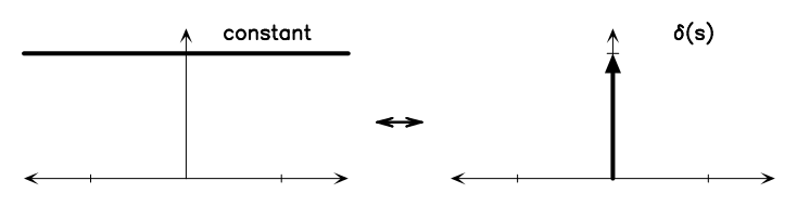
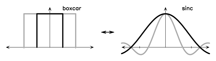
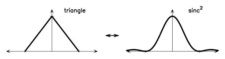
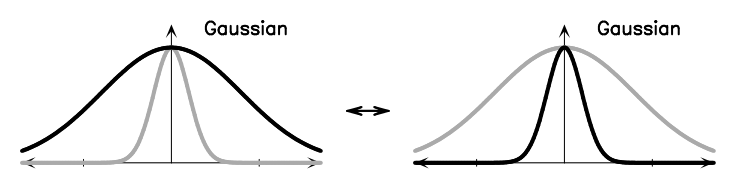
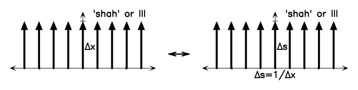
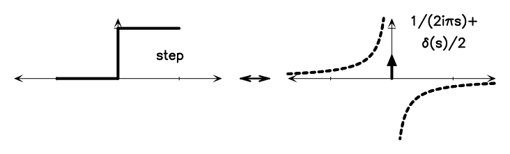
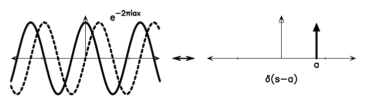
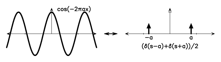
Figure A.1 shows some basic Fourier transform pairs. These can be combined using the Fourier transform theorems below to generate the Fourier transforms of many different functions. There is a nice Java applet⁵⁵ 5 http://webphysics.davidson.edu/Applets/mathapps/mathapps_fft.html. on the web that lets you experiment with various simple DFTs.

Convolution shows up in many aspects of astronomy, most notably in the point-source response of an imaging system and in interpolation. Convolution, which we will represent by $\ast$ (the symbol $\otimes$ is also frequently used for convolution), multiplies one function $f$ by the time-reversed kernel function $g$, shifts $g$ by some amount $u$, and integrates $u$ from $-\mathrm{\infty }$ to $+\mathrm{\infty }$. The convolution $h(x)$ of the functions $f$ and $g$ is a linear functional defined by

$$\boxed{h(x)=f\ast g\equiv {\int }_{-\mathrm{\infty }}^{\mathrm{\infty }}f(u)g(x-u)du.}$$

(A.14)

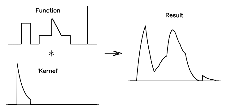
In Figure A.2, notice how the delta-function portion of the function produces an image of the kernel in the convolution. For a time series, that kernel defines the impulse response of the system. For an antenna or imaging system, the kernel is variously called the beam, the point-source response, or the point-spread function.

A very nice applet showing how convolution works is available online⁶⁶ 6 http://www.jhu.edu/~signals/convolve/index.html. (there is also a discrete version⁷⁷ 7 http://www.jhu.edu/~signals/discreteconv2/index.html.); a different visualization tool is also available. ⁸⁸ 8 https://maxwell.ict.griffith.edu.au/spl/Excalibar/Jtg/Conv.html.

The convolution theorem is extremely powerful and states that the Fourier transform of the convolution of two functions is the product of their individual Fourier transforms:

$$\boxed{f\ast g\iff F\cdot G.}$$

(A.15)

Cross-correlation is a very similar operation to convolution, except that the kernel is not time-reversed. Cross-correlation is used extensively in interferometry and aperture synthesis imaging, and is also used to perform optimal “matched filtering” of data to detect weak signals in noise. Cross-correlation is represented by the pentagram symbol $\star$ and defined by

$$\boxed{f\star g\equiv {\int }_{-\mathrm{\infty }}^{\mathrm{\infty }}f(u)g(u-x)du.}$$

(A.16)

In this case, unlike for convolution, $f(x)\star g(x)\ne g(x)\star f(x)$.

Closely related to the convolution theorem, the cross-correlation theorem states that the Fourier transform of the cross-correlation of two functions is equal to the product of the individual Fourier transforms, where one of them has been complex conjugated:

$$\boxed{f\star g\iff \overline{F}\cdot G.}$$

(A.17)

Autocorrelation is a special case of cross-correlation with $f\star f$. The related autocorrelation theorem is also known as the Wiener–Khinchin theorem and states

$$\boxed{f\star f\iff \overline{F}\cdot F=|F{|}^2.}$$

(A.18)

In words, the Fourier transform of an autocorrelation function is the power spectrum, or equivalently, the autocorrelation is the inverse Fourier transform of the power spectrum. Many radio-astronomy instruments compute power spectra using autocorrelations and this theorem. The following diagram summarizes the relations between a function, its Fourier transform, its autocorrelation, and its power spectrum:

One important thing to remember about convolution and correlation using DFTs is that they are cyclic with a period corresponding to the length of the longest component of the convolution or correlation. Unless this periodicity is taken into account (usually by zero-padding one of the input functions), the convolution or correlation will wrap around the ends and possibly “contaminate” the resulting function.

Of interest on the web, other Fourier-transform-related links include a Fourier series applet,⁹⁹ 9 http://www.jhu.edu/~signals/fourier2/index.html. some tones, harmonics, filtering, and sounds,¹⁰¹⁰ 10 http://www.jhu.edu/~signals/listen-new/listen-newindex.htm. and a nice online book on the mathematics of the DFT.¹¹¹¹ 11 http://ccrma.stanford.edu/~jos/mdft/mdft.html.