Next: Mapping the Jagiellonian Field of Galaxies
Previous: Imaging by an Optimizing Method
Up: Algorithms
Table of Contents - Index - PS reprint
Astronomical Data Analysis Software and Systems VI
ASP Conference Series, Vol. 125, 1997
Editors: Gareth Hunt and H. E. Payne
V. S. Shergin, O. V. Verkhodanov, V. N. Chernenkov, B. L. Erukhimov,
and V. L. Gorokhov
Special Astrophysical observatory, Nizhnij Arkhyz,
Karachaj-Cherkessia, Russia, 357147
Abstract:
Non-linear and non-parametric algorithms for data averaging,
smoothing and clipping in the RATAN-600 flexible astronomical
data processing system are proposed. Algorithms are based on
robust methods and non-linear filters using an iterative
approach to smoothing and clipping.
Using robust procedures to detect faint
sources is proposed also. This detector is based on the
ratio of two statistics, characterizing the noise and signal,
in the given interval.
These methods allow us to accelerate the process of the data
reduction and to improve the signal/noise ratio.
Examples of operation of these algorithms are shown.
Obtaining a reliable result on the background
from different types of interferences is one of the main
problems for the observational astronomy. The question ``what
is useful signal and what is noise?'' is especially
essential when we begin ``dumb'' data processing.
The ordinary way to obtain a good signal/noise ratio is to
apply the standard average for vectors of data observed
on the same sky strip. This way is the most optimal and
realizes the maximum likelihood estimation with  improvement. But the real observational data have a
distribution far from normal. This is caused by the presence
of power spikes, ``jumps,'' and slow trends. The source of this
interference is human activity, atmosphere, and possible
instability of the receiver. Therefore, observers prefer a manual
method of data reduction, because a single bad record spoils
the resulting sum when doing ``dumb'' standard averaging. To automate
the users' procedure of data quality checking, special
algorithms have been worked out.
The background problems are absent for ordinary average.
But when we use the robust (non-parametric)
average, the correct background subtraction
(or smoothing) is the main problem. Therefore,
the first problem to be solved is to find the correct (from the viewpoint
of an observer) smoothing. Moreover, the knowledge
about the background around the sources is very important
for some problems in radio astronomy.
The use of standard procedures (fitting with
splines) very often can not help us in this
situation. Thus, special non-linear
algorithms for smoothing were developed.
Another type of processing where similar algorithms
can be used is data compression (when we have a surplus of points
per beam and can compress the data keeping useful information)
and searching for sources.
The history of algorithms, based on
the robust methods and non-linear filters using an iterative
approach to smoothing and clipping, began twelve years ago
in the data reduction at the RATAN-600. Since then they have been
further developed and are used in modern computer systems
in the RATAN-600 data reduction system FADPS
(Verkhodanov et al. 1993; Verkhodanov 1997)
and in the MIDAS (Shergin et al. 1995).
The algorithm uses
several start parameters: noise dispersion, smoothing interval,
iteration count, and type of smoothing curve.
Practically there is no effect on a real signal
in a given interval, and the background is accurately calculated.
The detailed description of the smoothing and clipping (SAC)
algorithm is given in Erukhimov et al. (1990) and
in Shergin et al. (1996). Briefly, the SAC algorithm consists of
the following steps: (i) calculation of an input vector  for
for  -th smoothing iteration as
 where
where  is a vector of weights calculated in the
previous iteration. In the simplest case the function
  is calculated
as a product of each vector component
  ,
where k is k-th component; (ii) smoothing of
  :
:
 , where
 is the smoothing operator, and
 is the input parameter; (iii) subtraction
 , where
 is the input data vector; (iv)
calculation of a new function of weights as a non-linear transformation
 which is a function of input noise
  and
number of iteration in a general case:
 ; and (v) transition to
the next iteration. There are several
possible smoothing and weighting methods. In practice we use
the following methods for smoothing:
simple boxcar average;
convolution with Gaussian profile (see Figure 1 in Verkhodanov 1997),
median average (Erukhimov et al. 1990)
(see Figure 2 in Verkhodanov 1997);
weighted least squares polynomial approximation of 1/15°.
For calculation of weights some empirical transformations are used.
They may be specialized to cut emission, absorption or both.
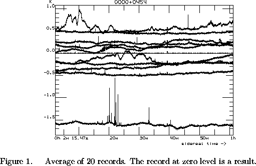
After background subtraction the procedure of robust averaging
is applied for records. Usually we do it by the Hodges-Lehmann (HL) method
(Huber 1981, Erukhimov et al. 1990) with estimation of middle value:

Robust averaging with the HL method is illustrated in Figure 1.
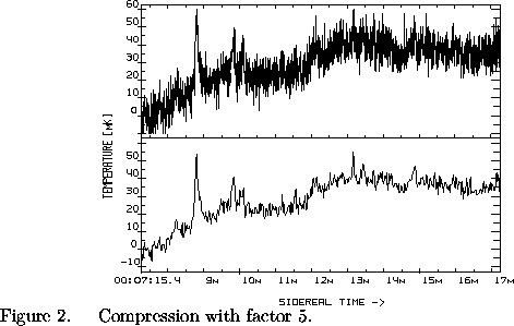
Another type of data reduction procedure is data compression.
The result of data compression on the base of Hodges-Lehmann
(Huber 1981) estimates is illustrated in Figure 2.
A similar robust algorithm was proposed and applied in the
RATAN-600 data registration system by Chernenkov (1996).
Based on robust procedures, a detector for faint
sources (extremal-median signal detector: EMSD)
in a series of synchronous scans (Verkhodanov & Gorokhov 1995).
is proposed also. This detector is based on the
ratio of two statistics, characterizing the noise and signal,
in the given interval.
For this algorithm several statistics are calculated:
 ,
,
 , where
  ;
D is the matrix of m vectors, m is the number of scans,
n is the number of points in a scan, r is the number of points in
a signal search interval. Using these two extremal
statistics the medians and the following statistics are computed in
each interval:
 ,
,
 , where
  ;
then their ratio is used as a test statistic:

where j=1,n.
In this case the hypothesis of object detection is adapted
when the quantity  exceeds a certain quantity
  .
The threshold
  can be either set by user or
computed in the program.
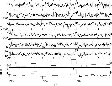
The example of EMSD operation is illustrated in Figure 3.

Figure:
Results of EMSD operation for the different input intervals:
g-interval of
two beam patterns, h-one beam pattern, for real data of five
synchronous scans (a-e). To compare results the scan with robust
average of these data is shown (f). The antenna temperature is
for the first six scans, and ratio (5) is for the two last scans
plotted along the Y-axis.
Original PostScript figure (68kB).
Acknowledgments:
O. Verkhodanov thanks ISF-LOGOVAZ Foundation for the travel grant,
the SOC for the financial aid in the living expenses and
the LOC for the hospitality.
References:
Chernenkov, V. N. 1996, Bull. of SAO, 41, 150
Erukhimov, B. L., Vitkovskij, V. V., & Shergin, V. S. 1990,
Preprint SAO RAS, 50
Huber, P. J. 1981, Robust Statistics (New York: Wiley)
Shergin, V. S., Kniazev, A. Yu., & Lipovetsky, V. A. 1996, Astron.
Nach., 317, 95
Verkhodanov, O. V., Erukhimov, B. L., Monosov, M. L., Chernenkov, V. N.,
& Shergin, V. S. 1993, Bull. of SAO, 36, 132
Verkhodanov, O. V., & Gorokhov, V. L. 1995, Bull. of SAO,
39, 155
Verkhodanov, O. V. 1997, this volume
© Copyright 1997 Astronomical Society of the Pacific,
390 Ashton Avenue, San Francisco, California 94112, USA
Next: Mapping the Jagiellonian Field of Galaxies
Previous: Imaging by an Optimizing Method
Up: Algorithms
Table of Contents - Index - PS reprint
payne@stsci.edu
 improvement. But the real observational data have a
distribution far from normal. This is caused by the presence
of power spikes, ``jumps,'' and slow trends. The source of this
interference is human activity, atmosphere, and possible
instability of the receiver. Therefore, observers prefer a manual
method of data reduction, because a single bad record spoils
the resulting sum when doing ``dumb'' standard averaging. To automate
the users' procedure of data quality checking, special
algorithms have been worked out.
 for
for  -th smoothing iteration as
 where
where  is a vector of weights calculated in the
previous iteration. In the simplest case the function
  is calculated
as a product of each vector component
  ,
where k is k-th component; (ii) smoothing of
  :
:
 , where
 is the smoothing operator, and
 is the input parameter; (iii) subtraction
 , where
 is the input data vector; (iv)
calculation of a new function of weights as a non-linear transformation
 which is a function of input noise
  and
number of iteration in a general case:
 ; and (v) transition to
the next iteration. There are several
possible smoothing and weighting methods. In practice we use
the following methods for smoothing:
simple boxcar average;
convolution with Gaussian profile (see Figure 1 in Verkhodanov 1997),
median average (Erukhimov et al. 1990)
(see Figure 2 in Verkhodanov 1997);
weighted least squares polynomial approximation of 1/15°.
For calculation of weights some empirical transformations are used.
They may be specialized to cut emission, absorption or both.


 ,
,
 , where
  ;
D is the matrix of m vectors, m is the number of scans,
n is the number of points in a scan, r is the number of points in
a signal search interval. Using these two extremal
statistics the medians and the following statistics are computed in
each interval:
 ,
,
 , where
  ;
then their ratio is used as a test statistic:

 exceeds a certain quantity
  .
The threshold
  can be either set by user or
computed in the program.
The example of EMSD operation is illustrated in Figure 3.
