Chapter 3 Radio Telescopes and Radiometers
3.1 Antenna Fundamentals
An antenna is a passive device that converts electromagnetic radiation in space into electrical currents in conductors or vice versa, depending on whether it is being used for receiving or for transmitting, respectively. Radio telescopes are receiving antennas, and radar telescopes are also transmitting antennas. It is often easier to calculate the properties of transmitting antennas and to measure the properties of receiving antennas. Fortunately, most characteristics of a transmitting antenna (e.g., its radiation pattern) are unchanged when that antenna is used for receiving, so any analysis of a transmitting antenna can be applied to a receiving antenna used in radio astronomy, and any measurement of a receiving antenna can be applied to that antenna when used for transmitting.
3.1.1 Radiation from a Short Dipole Antenna (Hertz Dipole)

The simplest antenna is a short (total length much smaller than one wavelength ) dipole antenna, which is shown in Figure 3.1 as two collinear conductors (e.g., wires or conducting rods). When they are driven at the small gap between them by an oscillating current source (a transmitter), the current going into the bottom conductor is 180 degrees out of phase with the current going into the top conductor. The radiation from a dipole depends on the transmitter frequency, so consider a sinusoidal driving current with angular frequency :
| (3.1) |
where is the peak current going into each half of the dipole. It is computationally convenient to replace the trigonometric function with its complex exponential equivalent (Appendix B.3), the real part of
| (3.2) |
so the driving current can be rewritten as
| (3.3) |
with the implicit understanding that only the real part of represents the actual current. The driving current accelerates charges in the antenna wires, so Larmor’s formula can be used to calculate the radiation from the antenna by converting from charges and accelerations to time-varying currents.
The electric current in a wire is defined as the flow rate of electric charge along the wire:
| (3.4) |
For a wire on the -axis,
| (3.5) |
where is the instantaneous flow velocity of the charges.
Many people incorrectly believe that the velocity of individual electrons in a wire is comparable with the speed of light because electrical signals do travel down wires at nearly the speed of light. However, a wire filled with electrons is like a garden hose already filled with water, a nearly incompressible fluid. When the faucet is turned on, water flows from the other end of a full hose almost immediately, even though individual water molecules have moved only a short distance along the hose. The example above shows that electrons move so slowly in a wire that Larmor’s nonrelativistic equation accurately predicts the radiation from antennas.
Equation 2.136 from the derivation of Larmor’s formula
can be applied to yield the contributed by each infinitesimal dipole segment of length . If the dipole is short (), all of these electric fields are in phase and add directly to give the total produced by the dipole:
| (3.6) |
At distances , () is nearly constant over the whole antenna and can be taken outside the integral. For a sinusoidal driving current, and
| (3.7) |
That is, the radiated electric field strength is proportional to the integral of the current distribution along the antenna. The current at the center is the driving current , and the current must drop to zero at the ends of the antenna, where the conductivity goes to zero. The current distribution along a short dipole is the tail end of a standing-wave sinusoid, which declines almost linearly from the driving current at the center to zero at the ends:
| (3.8) |
Then
| (3.9) |
and
| (3.10) |
Substituting gives
| (3.11) |
The time-averaged Poynting flux (power per unit area) follows from Equation 2.139; it is
| (3.12) |
Thus
| (3.13) |
where the factor reflects the fact that . (This is a good relation to remember and an easy one to derive because and .)
The power pattern of a transmitting antenna is the angular distribution of its radiated power, often normalized to unity at the peak. From Equation 3.13 the normalized power pattern of a short dipole is
| (3.14) |
The radiation from a short dipole has the same polarization and the same doughnut-shaped power pattern as Larmor radiation from an accelerated charge because all of the charges in the short dipole are being accelerated along one line much shorter than one wavelength. From the observer’s point of view, the power received depends only on the projected (perpendicular to the line of sight) length of the dipole. The electric field strength received is proportional to the apparent length of the dipole, and the radiation from the dipole is linearly polarized parallel to the projected dipole. The time-averaged total power emitted is obtained by integrating the Poynting flux over the surface area of a sphere of any radius centered on the antenna:
| (3.15) | ||||
| (3.16) |
Recall that , so the time-averaged power radiated by a short dipole is
| (3.17) |
where is the driving current and is the total length of the dipole in wavelengths.
Most practical dipoles are half-wave dipoles () because half-wave dipoles are resonant, meaning that they provide a nearly resistive load to the transmitter. When each half of the dipole is long, the standing-wave current is highest at the center and naturally falls as to zero at the ends of the conductors.
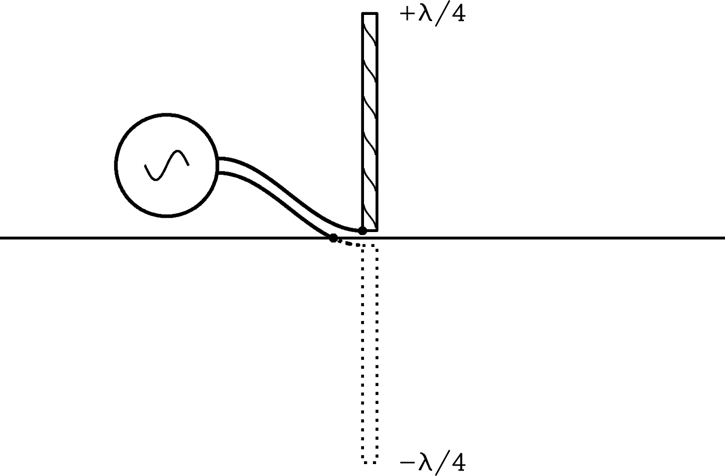
The ground-plane vertical antenna shown in Figure 3.2 is very similar to the dipole. A ground-plane vertical is one half of a dipole above a conducting plane, which is called a “ground plane” because historically the conducting plane for vertical antennas was the surface of the Earth. The transmitter is connected between the base of the vertical, which is insulated from the ground, and the ground plane near the base. Many AM broadcast transmitting antennas are tall (at MHz, m and a vertical antenna is about 75 m high), insulated towers acting as quarter-wave verticals. The conducting ground plane is a mirror that creates the lower half of the dipole as the mirror image of the upper half. Electric fields produced by the vertical antenna induce currents in the conducting plane to make the horizontal component of the electric field go to zero on the conductor. The virtual electric fields from the image vertical have the same amplitude but are 180 degrees out of phase, exactly as in a half-wave dipole. Consequently the radiation field from a ground-plane vertical is identical to that of a dipole in the half space above the ground plane and zero below the ground plane.
According to the strict definition of an antenna as a device for converting between electromagnetic waves in space and currents in conductors, the only antennas in most radio telescopes are half-wave dipoles and their relatives, quarter-wave ground-plane verticals. The large parabolic reflector of a radio telescope serves only to focus plane waves onto the feed antenna. (The term “feed” comes from radar antennas used for transmitting; the “feed” antenna feeds transmitter power to the main reflector. Receiving antennas used in radio astronomy work the other way around, and the “feed” actually collects radiation from the reflector.)
Actual half-wave dipoles, backed by small reflectors about behind them to focus the dipole pattern in the direction of the main dish, are normally used as feeds at low frequencies ( GHz) or long wavelengths ( m) because of their relatively small size. However, the radiation patterns of half-wave dipoles backed by small reflectors are not well matched to most parabolic dishes, so their performance is less than optimum.
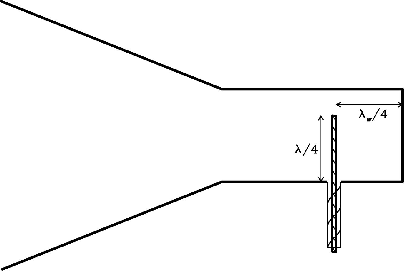
For shorter wavelengths, almost all radio-telescope feeds are quarter-wave ground-plane verticals inside waveguide horns. Radiation entering the relatively large (size ) rectangular or circular aperture of the tapered horn is concentrated into a rectangular or circular waveguide with parallel conducting walls. In the case of the rectangular waveguide whose cross section is shown in Figure 3.3, the side walls are separated by slightly over so that vertical electric fields can travel down the waveguide with low loss. The top and bottom walls are separated by somewhat less than so only the mode with vertical electric fields can propagate (Section 3.4). The vertical antenna inserted through a small hole in the bottom wall collects most of this vertically polarized radiation and converts it into an electric current that travels down the coaxial cable to the receiver. The backshort wall about 1/4 of the guide wavelength (Equation 3.144) behind the dipole ensures that the dipole sees only radiation coming from the direction of the horn opening.
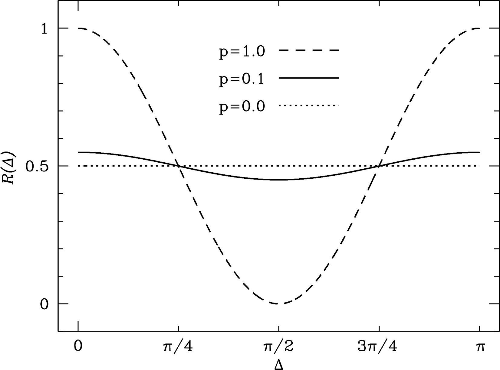
Both dipoles and quarter-wave verticals are linearly polarized feeds. The voltage response of a linearly polarized feed to a linearly polarized source is proportional to , where is the angle between the feed and the source electric field, and the power response is proportional to . Consequently the degree of polarization and the polarization position angle of a partially linearly polarized radio source can be measured by rotating the linearly polarized feed of a radio telescope while tracking the source. The degree of polarization of a partially linearly polarized source defined by Equation 2.58 is
| (3.18) |
where is the polarized flux density and is the total flux density of the source. The power response of the feed will be when the feed and source polarizations are parallel () and when they are perpendicular (). In terms of the observables and , the degree of polarization is
| (3.19) |
Figure 3.4 shows how the relative power output of a linearly polarized feed varies as it is rotated through radians relative to the polarization position angle of sources with fractional polarizations , 0.1, and 0.0.
To measure all four Stokes parameters of an arbitrarily polarized source, it is necessary to combine the voltage outputs of two orthogonally polarized feeds. For example, two orthogonal quarter-wave verticals can be inserted into a square waveguide to receive both the horizontally and the vertically polarized components simultaneously. If their output voltages are added in phase (phase difference in Figure 2.15), the feed combination will respond to radiation linearly polarized in position angle . If a phase difference is inserted either mechanically (by moving one feed behind the other) or electrically (by inserting a longer cable between one feed and the point where the two outputs are added), then and the feed combination will respond to circular polarization.
3.1.2 Radiation Resistance
The power flowing through a circuit is
| (3.20) |
where is the voltage (defined as energy per unit charge) and is the current (defined as the charge flowing through the circuit per unit time), so has dimensions of energy per unit time. The physicist George Simon Ohm observed that the current flowing through most (but not all) materials is proportional to the applied voltage, so most objects have a well-defined resistance defined by Ohm’s law,
| (3.21) |
When Ohm’s law holds,
| (3.22) |
The average power in a resistive circuit with time-varying currents is
| (3.23) |
In the particular case of sinusoidal currents and , so
| (3.24) |
Thus the (frequency-dependent) radiation resistance of an antenna is defined by
| (3.25) |
For a short dipole, the power emitted is given by Equation 3.17 and the radiation resistance is
| (3.26) |
Example. A “half-wave” (length ) dipole is a resonant antenna. Resonant antennas are used in most real applications because the impedance of a resonant antenna is resistive; nonresonant antennas have large capacitive or inductive reactances as well. Most of the antenna current in a half-wave dipole is a standing wave with a current distribution that has a maximum at the feed point and declines co-sinusoidally to zero at the endpoints . With the (no longer so accurate) assumption that the radiation from all parts of the dipole emit in phase, Equation 3.7 still holds:
The current distribution of the half-wave dipole is
so
which is a factor of larger than the comparable integral for a short dipole (Equation 3.8):
The average power radiated by a given is proportional to the square of this factor (see Equations 3.10 through 3.17), or
Thus the radiation resistance of a half-wave dipole is the radiation resistance of a short dipole (Equation 3.26) multiplied by the factor squared:
Engineers and real test instruments use the MKS “ohm” (symbol ) as the unit of resistance. The conversion factor is 1 = , so
This is pretty close to the result from an exact calculation that doesn’t use the approximation.
A ground-plane vertical of height emits exactly like a dipole of length above the ground plane and nothing below the ground plane. Thus the total power emitted by the vertical is half the power emitted by the dipole, and the radiation resistance of the vertical is half the radiation resistance of the dipole.
The radiation resistance of free space (sometimes called the impedance of free space) can be obtained from the relations
| (3.27) |
The electric field is just the voltage per unit length and the flux is the power per unit area , so
| (3.28) |
and
| (3.29) |
Converting from CGS to MKS units yields the radiation resistance of space in ohms:
| (3.30) |
The tapered opening of a waveguide horn feed (Figure 3.3) acts as an impedance transformer to match the impedance of the waveguide to the impedance of free space to minimize standing waves and couple power efficiently between the waveguide and space, just as the bell of a trombone is an acoustic transformer matching sound vibrations of air in the trombone to the outside environment.
A black hole is a perfect absorber of radiation, so its resistance must also be to match that of free space. A black hole spinning in an external magnetic field can generate electrical power with a voltage/current ratio of , and this process may be important in powering quasar jets [12].
3.1.3 The Power Gain of a Transmitting Antenna
The power gain of a transmitting antenna is defined as the power transmitted per unit solid angle in direction relative to an isotropic antenna, which has the same gain in all directions. Frequently, the value of is expressed logarithmically in units of decibels (dB):
| (3.31) |
For any lossless antenna, energy conservation requires that the gain averaged over all directions be
| (3.32) |
Consequently, all lossless antennas obey
| (3.33) |
Different lossless antennas may radiate with different directional patterns, but they do not alter the total amount of power radiated. Consequently, the gain of a lossless antenna depends only on the angular distribution of radiation from that antenna. In general, an antenna having peak gain must beam most of its power into a solid angle such that . This motivates the definition of the beam solid angle :
| (3.34) |
Thus the higher the gain, the smaller the beam solid angle.
The antenna efficiency is defined as the ratio of radiated power to input power. If ohmic losses reduce , then the gain in Equations 3.31 through 3.34 should be replaced by the directivity defined by .
3.1.4 The Effective Area of a Receiving Antenna
The receiving counterpart of transmitting power gain is the effective area or effective collecting area of a receiving antenna. Imagine an ideal antenna of geometric area that could collect all of the radiation falling on it from a distant point source and convert it to electrical power—a “rain gauge” for collecting photons. The total spectral power incident on the antenna is the product of its geometric area and the incident spectral power per unit area, or flux density . However, any single antenna can respond to only one polarization, so its output can equal all of the input spectral power () from a fully polarized source whose polarization matches that of the antenna, but only half of the incident power () from an unpolarized source and nothing at all from an orthogonally polarized source. The output of a real antenna is always smaller than this and most radio sources are nearly unpolarized, so radio astronomers find it useful to define the effective collecting area of an antenna whose output spectral power is in response to an unpolarized point source of total flux density by
| (3.35) |
The average collecting area
| (3.36) |
of any lossless antenna can be calculated via another thermodynamic thought experiment.
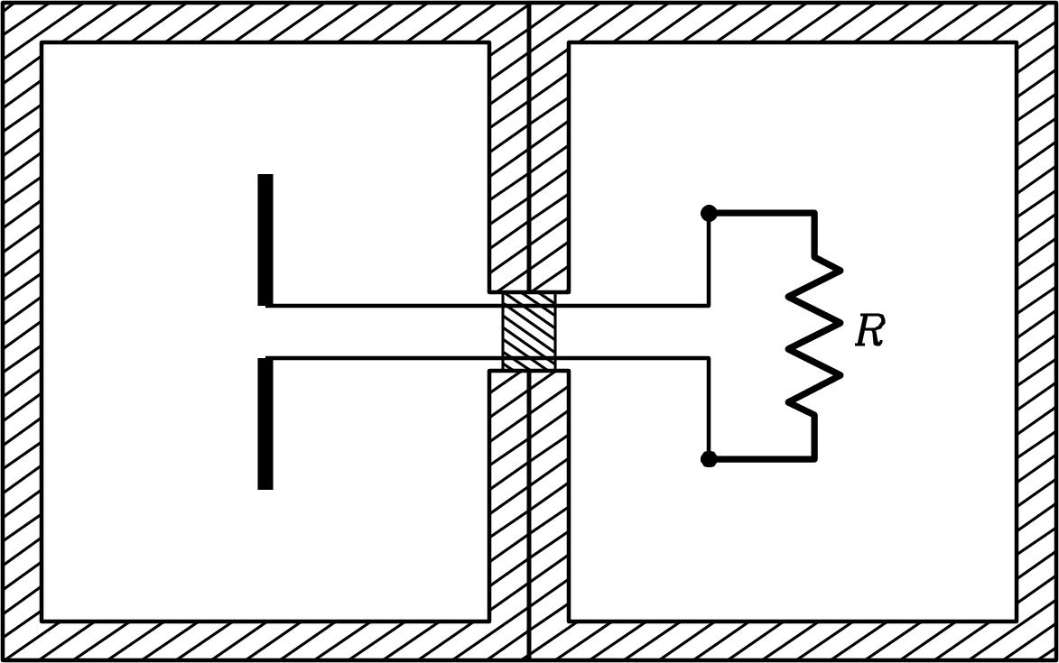
Imagine an antenna inside a cavity in full thermodynamic equilibrium at temperature connected through a transmission line to a matched resistor (whose resistance equals the radiation resistance of the antenna) in a second cavity at the same temperature (Figure 3.5). A filter between the cavities passes only currents in a narrow range of frequencies between and . Because this entire system is in thermodynamic equilibrium, no net power can flow through the wires connecting the antenna and the resistor. Otherwise, one cavity would heat up and the other would cool down, in violation of the second law of thermodynamics. The total spectral power from all directions collected in one polarization is half the total spectral power in the unpolarized blackbody radiation, so
| (3.37) |
must equal the Nyquist spectral power produced by the resistor. Inserting the Nyquist formula from Equation 2.119 and Planck’s law from Equation 2.85,
| (3.38) |
leads to
| (3.39) |
and finally,
| (3.40) |
Without using Maxwell’s equations we have obtained the remarkable result
| (3.41) |
which implies that all lossless antennas, from tiny dipoles to the 100-m diameter Green Bank Telescope (GBT), have the same average collecting area. is proportional to because space has two more dimensions than a transmission line has.
The collecting area of an isotropic receiving antenna is proportional to , so most satellite broadcast services, GPS (Global Positioning System) or satellite FM radio for example, operate at relatively long wavelengths (10 to 20 cm). Likewise, practical radio telescopes constructed from arrays of dipoles are reasonably sensitive only at long wavelengths.
By analogy with Equation 3.34, the beam solid angle of a lossless receiving antenna is defined as
| (3.42) |
where is the maximum effective collecting area, so
| (3.43) |
The much larger peak collecting area of the GBT implies it has a much smaller beam solid angle .
3.1.5 Reciprocity Theorems
Many antenna properties are the same for both transmitting and receiving. It is often easier to calculate the gain of a transmitting antenna than the collecting area of a receiving antenna, and it is often easier to measure the receiving power pattern of a large radio telescope than to measure its transmitting power pattern. Thus this receiving/transmitting “reciprocity” greatly simplifies antenna calculations and measurements. Reciprocity can be understood via Maxwell’s equations or by thermodynamic arguments.
Burke and Graham-Smith [20] state the electromagnetic case for reciprocity clearly: “An antenna can be treated either as a receiving device, gathering the incoming radiation field and conducting electrical signals to the output terminals, or as a transmitting system, launching electromagnetic waves outward. These two cases are equivalent because of time reversibility: the solutions of Maxwell’s equations are valid when time is reversed.”
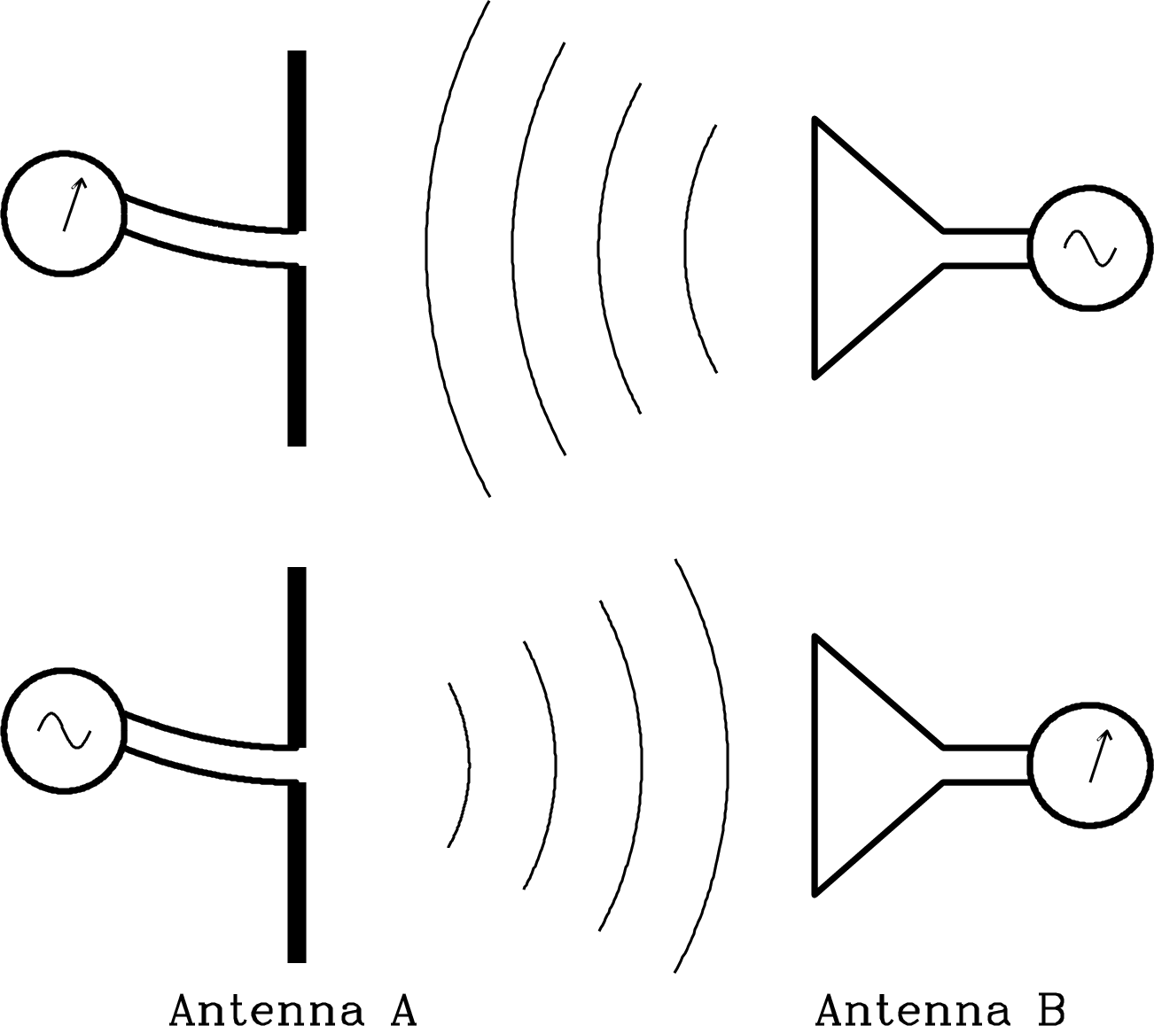
The strong reciprocity theorem states,
If a voltage is applied to the terminals of an antenna A and the current is measured at the terminals of another antenna B, then an equal current (in both amplitude and phase) will appear at the terminals of A if the same voltage is applied to B. (Figure 3.6)
It can be formally derived from Maxwell’s equations (see a partial derivation in Wilson et al. [116, Appendix D]) or by network analysis (see Kraus et al. [63, “Antennas”, p. 252]).
Most radio astronomical applications do not depend on the detailed phase relationships of voltages and currents, so it is sufficient to use a weak reciprocity theorem that relates the angular dependences of the transmitting power pattern and the receiving collecting area of any antenna: “The power pattern of an antenna is the same for transmitting and receiving”; that is,
| (3.44) |
The weak reciprocity theorem can be proven by another simple thermodynamic thought experiment: An antenna is connected to a matched load inside a cavity initially in equilibrium at temperature . The antenna simultaneously receives power from the cavity walls and transmits power generated by the resistor. The total power transmitted in all directions must equal the total power received from all directions because no net power can be transferred between the antenna and the resistor; otherwise the resistor would not remain at temperature . Moreover, in any direction, the power received and transmitted by the antenna must be the same, else the cavity wall in directions where the transmitted power was greater than the received power would rise in temperature and the cavity wall in directions of lower transmitted/received power ratio would cool, leading to a violation of the second law of thermodynamics.
Thus energy conservation and the weak reciprocity theorem imply
| (3.46) |
for any antenna. This extremely useful equation shows how to compute the receiving power pattern from the transmitting power pattern and vice versa.
3.1.6 Antenna Temperature
A convenient practical unit for the power output per unit frequency from a receiving antenna is the antenna temperature . Antenna temperature has nothing to do with the physical temperature of the antenna as measured by a thermometer; it is only the temperature of a matched resistor whose thermally generated power per unit frequency in the low-frequency Nyquist approximation (Equation 2.117) equals that produced by the antenna:
| (3.47) |
It is widely used for the following reasons:
-
1.
1 K of antenna temperature is a conveniently small power per unit bandwidth. K corresponds to .
-
2.
It can be calibrated by a direct comparison with hot and cold loads (another word for matched resistors) connected to the receiver input.
-
3.
The units of receiver noise are also K, so comparing the signal in K with the receiver noise in K makes it easy to compare the signal and noise powers.
Combining Equations 3.35 and 3.47 shows that an unpolarized point source of flux density increases the antenna temperature by
| (3.48) |
where is the effective collecting area. It is often convenient to express the point-source sensitivity of a radio telescope in units of “kelvins per jansky” rather than in units of effective collecting area (m). The effective collecting area corresponding to a sensitivity of is
| (3.49) |
In an arbitrary radiation field , Equation 3.37 becomes
| (3.50) |
Replacing by antenna temperature using Equation 3.47 and inserting (Equation 2.33) gives
| (3.51) | ||||
| (3.52) |
In the limit of a very extended source having nearly constant across the entire beam,
| (3.53) |
so
| (3.54) |
In words, the antenna temperature produced by a smooth source much larger than the antenna beam equals the source brightness temperature.
If a lossless antenna is pointed at a compact source covering a solid angle much smaller than the beam and having uniform brightness temperature , then
| (3.55) |
where is the on-axis effective collecting area. Substituting (Equation 3.43) gives the result:
| (3.56) |
Stated in words, the antenna temperature equals the source brightness temperature multiplied by the fraction of the beam solid angle filled by the source. A K source covering 1% of the beam solid angle will add 100 K to the antenna temperature. The ratio is called the beam filling factor.
The main beam of an antenna is defined as the region containing the principal response out to the first zero; responses outside this region are called sidelobes or, very far from the main beam, stray radiation. The main beam solid angle is defined as
| (3.57) |
The fraction of the total beam solid angle lying inside the main beam is called the main beam efficiency or, loosely, the beam efficiency:
| (3.58) |
3.2 Reflector Antennas
3.2.1 Paraboloidal Reflectors
Antennas useful for radio astronomy at short wavelengths must have collecting areas much larger than the collecting area of an isotropic antenna and much higher angular resolution than a short dipole provides. Because arrays of dipoles are impractical at wavelengths m or so, most radio telescopes use large reflectors to collect and focus power onto their small feed antennas, such as waveguide horns or dipoles backed by small reflectors, that are connected to receivers. The most common reflector shape is a paraboloid of revolution because it can focus the plane wave from a distant point source onto a single focal point.
To focus plane waves onto a single point, the reflector must keep all parts of an on-axis plane wavefront in phase at its focal point. Thus the total path lengths to the focus must all be the same, and this requirement is sufficient to determine the shape of the desired reflecting surface. Clearly the surface must be rotationally symmetric about its axis. In any plane containing the axis, the surface looks like the curve in Figure 3.7.
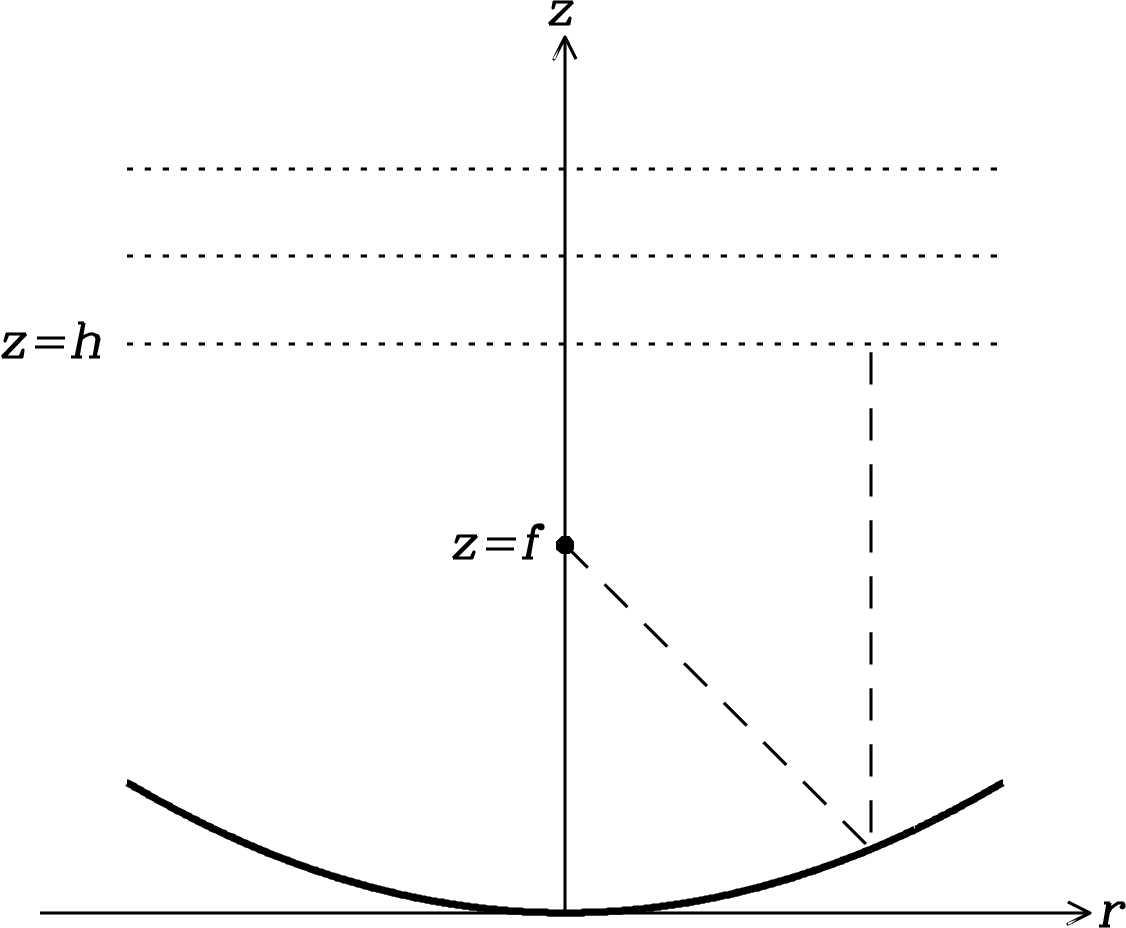
The requirement of constant path length can be written by equating the on-axis path length from any height to the reflector and then back to the prime focus at height with the off-axis path length:
| (3.59) |
This yields the reflector height as a function of radius :
the result is
| (3.60) |
This is the equation of a paraboloid with focal length .
The ratio of the focal length to the diameter of the reflector is called the ratio or focal ratio. Note that the gain, collecting area, and beamwidth of a reflector antenna depend only weakly and indirectly on , via the effect of on illumination taper. In principle, is a free parameter for the telescope designer, but in practice it is constrained. If the reflector is too high, the support structure needed to hold the feed or subreflector at the focus of a large radio telescope becomes very long and unwieldy. Consequently large radio telescopes usually have , an order-of-magnitude lower than the typical focal ratio of an optical telescope. The drawback of a low is a small field of view. The focal ellipsoid is the volume around the exact focal point that remains in reasonably good focus, and the focal circle is defined by the intersection of the focal ellipse and the transverse plane at . Ruze [96] showed that the angular radius of the focal circle is proportional to , and only a small number (about seven) of discrete feeds can fit inside the focal circle of an paraboloid. Large arrays of feeds or imaging cameras require larger ratios, obtained either by using a shallower paraboloid or by using magnifying subreflectors to increase the effective focal length.
The primary mirrors of most radio telescopes are circular paraboloids or sections thereof for the following reasons:
-
1.
The effective collecting area of a reflector antenna can approach its projected geometric area .
-
2.
They are electrically simple (compared with a phased array of dipoles, for example).
-
3.
A single reflector can work over a wide range of frequencies. Changing frequencies only requires changing the feed antenna and receiver located at the focal point, not building a whole new radio telescope.
3.2.2 The Far-Field Distance
How far away must a point source be for the received waves to satisfy the assumption that they are nearly planar across the reflector? The answer depends on both the wavelength and the reflector diameter . Figure 3.8 shows the spherical wave emitted by a point source a finite distance from a flat aperture, an imaginary circular hole that covers the reflector. It could be located at the plane shown in Figure 3.7, for example.
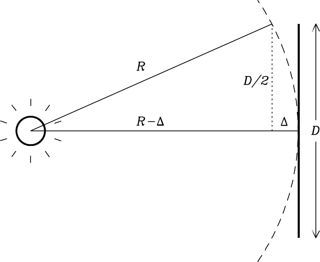
The maximum departure from a plane wave occurs at the edge of the aperture. The far-field distance is somewhat arbitrarily defined by requiring that . At the aperture edge, the Pythagorean theorem gives
| (3.61) |
Thus
| (3.62) |
In the limit , we have and
| (3.63) |
Given the criterion, the far-field distance is
| (3.64) |
If , the path-length errors will introduce significant phase errors in the waves coming from the off-axis portions of the reflector, reducing the effective collecting area and degrading the antenna pattern.
3.2.3 Patterns of Aperture Antennas
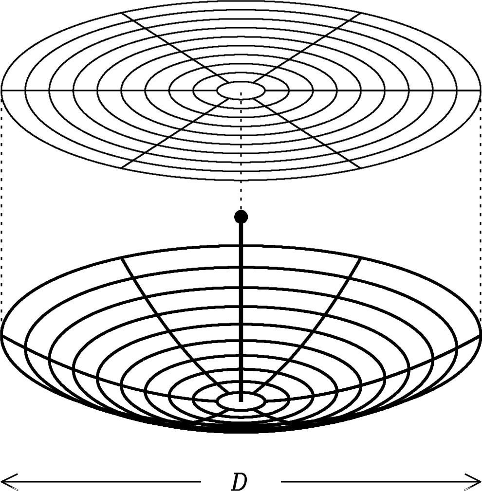
In optics, the term aperture refers to the opening through which all rays pass. For example, the aperture of a paraboloidal reflector antenna would be the plane circle, normal to the rays from a distant point source, that just covers the paraboloid (Figure 3.9). The phase of the plane wave from a distant point source would be constant across the aperture plane when the aperture is perpendicular to the line of sight.
Another example of an aperture is the mouth of a waveguide horn antenna (Figure 3.10).
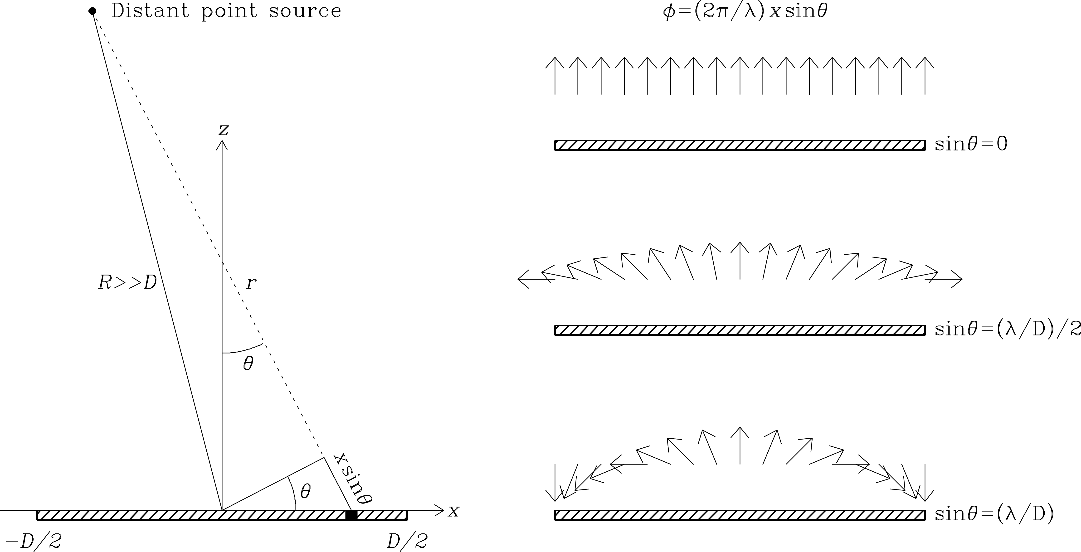
How can the beam pattern, or power gain as a function of direction, of an aperture antenna be calculated? For simplicity, first consider a one-dimensional aperture of width (Figure 3.11) and calculate the electric field pattern at a distant () point.
When used in a transmitting antenna, the feed can illuminate the aperture antenna with a sine wave of fixed frequency and electric field strength that varies across the aperture. The illumination induces currents in the reflector. The currents will vary with both position and time:
| (3.65) |
The constant of proportionality doesn’t matter yet; it can be calculated later from energy conservation. Huygens’s principle asserts that the aperture can be treated as a collection of small elements which act individually as small antennas. Huygens’s principle actually applies to waves of any type, sound waves for example. The electric field produced by the whole aperture at large distances is just the vector sum of the elemental electric fields from these small antennas. The field from each element extending from to is
| (3.66) |
where is the distance between the source and the aperture element at position (Figure 3.11). In the far field (Equation 3.64), the Fraunhofer approximation
| (3.67) |
is valid. This equation is usually written in the form
| (3.68) |
where
| (3.69) |
For the small angles rad relevant to large apertures, .
At large distances, the quantity
| (3.70) |
is nearly constant across the aperture and can be absorbed by the constant of proportionality in Equation 3.66. Although is a constant because is fixed, the variable part of in the numerator of Equation 3.66 cannot be ignored at any distance:
| (3.71) |
When the phase varies linearly across the aperture, and different parts of the aperture add constructively or destructively to the total electric field . Defining
| (3.72) |
to express position along the aperture in units of wavelength yields
| (3.73) |
In words, this very important equation says that in the far field, the electric-field pattern of an aperture antenna is the Fourier transform (Appendix A.1) of the electric field distribution illuminating that aperture.
3.2.4 The Electric-Field and Power Patterns of a Uniformly Illuminated Aperture
What is the electric-field pattern of a uniformly illuminated one-dimensional aperture of width at wavelength ? Uniform illumination means that the strength of the illumination is constant over the aperture:
This question is best answered in two steps: first find the far-field pattern of a unit aperture () and then use the similarity theorem (Equation A.11) for Fourier transforms to scale the first result to an aperture of any size.
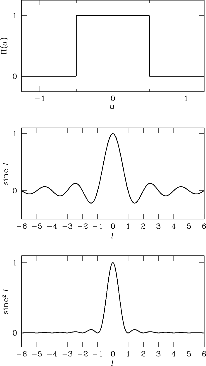
The unit rectangle function is defined as
| (3.74) |
and otherwise. The function symbol (an uppercase pi) is easy to remember because it looks like the function graph shown in the top panel of Figure 3.12.
Inserting into Equation 3.73 gives the field pattern of the uniformly illuminated unit aperture:
| (3.75) |
Thus
| (3.76) |
Next, difference the mathematical identities (Appendix B.3)
to derive
Inserting this result into Equation 3.76 gives
| (3.77) |
The useful sinc function defined in Equation 3.77 is plotted in the middle panel of Figure 3.12.
The power pattern is the square of the field pattern . The power pattern of a uniformly illuminated unit aperture is graphed in the bottom panel of Figure 3.12. The central peak of the power pattern between the first zeros at is called the main beam. The smaller peaks are called sidelobes. They are separated by zeros or nulls in the power pattern at
Next apply the powerful similarity theorem for Fourier transforms: if is the Fourier transform of , then
is the Fourier transform of , where is a dimensionless scaling factor. According to the similarity theorem, making a function wider () or narrower () makes its Fourier transform narrower and taller, or wider and shorter, respectively, always conserving the area under the transform. Consequently the beamwidth of an aperture antenna is inversely proportional to the aperture size in wavelengths and the on-axis field strength is directly proportional to the aperture size in wavelengths.
The scale factor for a uniformly illuminated one-dimensional aperture of width operating at wavelength is , so the electric field pattern becomes
If the aperture is large (), the relevant angles are so small ( radian) that and
| (3.78) |
The power pattern is proportional to the square of the electric field pattern, so
If radian, then
| (3.79) |
Radio astronomers use the angle between the half-power points to specify the angular width of the main beam, calling it the half-power beamwidth (HPBW) or the full width between half-maximum points (FWHM). The narrow beamwidth of a large () one-dimensional uniformly illuminated aperture satisfies
| (3.80) | |||
| (3.81) | |||
| (3.82) |
The similarity theorem implies the general scaling relation
| (3.83) |
The constant of proportionality varies slightly with the illumination taper. Even an ideal aperture antenna of finite size has a finite resolving power that is limited by diffraction, the spreading of rays passing through a finite aperture, and Equation 3.82 specifies the diffraction-limited resolution of a uniformly illuminated aperture antenna.
The weak reciprocity theorem (Section 3.1.5) says that the preceding analysis of the transmitting power pattern of an aperture antenna also yields its receiving power pattern, or the variation of with orientation. In receiving terms, the analog of the power pattern is called the point-source response. For a uniformly illuminated aperture, scanning a radio telescope beam in angle across a point source will cause the antenna temperature to vary as , and the width of the half-power response will equal the transmitting HPBW. The receiving HPBW is sometimes called the resolving power of a telescope because two equal point sources separated by the HPBW are just resolved by the Rayleigh criterion that the total response has a slight minimum midway between the point sources.
3.2.5 The Electric-Field and Power Patterns with Tapered Illumination
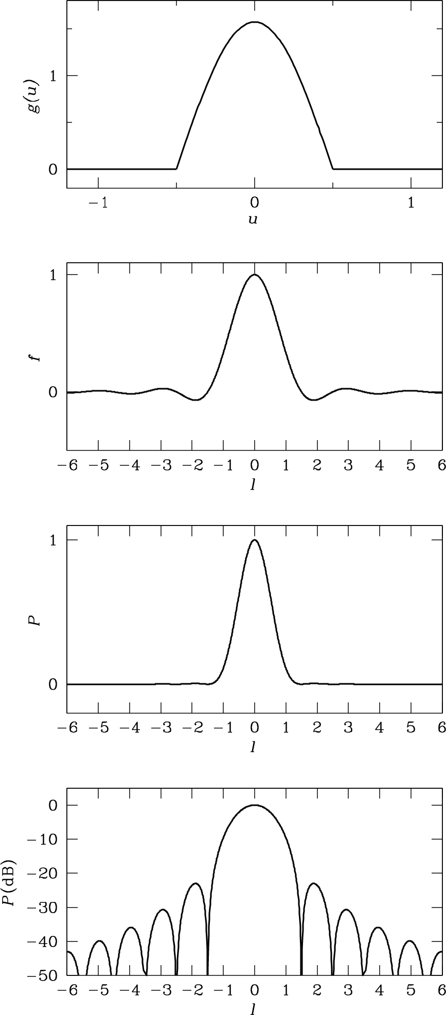
Practical feeds such as small waveguide horns or half-wave dipoles backed by small subreflectors cannot illuminate a large aperture uniformly. A better approximation to their illumination is the cosine-tapered field pattern (cosine-squared tapered power pattern)
| (3.84) |
and otherwise (Figure 3.13). The () normalization factor in Equation 3.84 ensures that
| (3.85) |
The corresponding field pattern of a one-dimensional unit aperture is given by
| (3.86) |
This Fourier transform can be evaluated as follows:
| (3.87) | ||||
| (3.88) | ||||
| (3.89) | ||||
| (3.90) | ||||
| (3.91) |
to yield the field pattern
| (3.92) |
of a one-dimensional unit aperture with cosine-tapered illumination given by Equation 3.84. Both the field pattern and the power pattern
| (3.93) |
are shown in Figure 3.13. The sidelobes are so weak that a plot of is needed to show them clearly (bottom panel of Figure 3.13).
Tapering increases the half-power beamwidth. If , the normalized power pattern is
| (3.94) |
and
| (3.95) |
can be solved numerically to yield
| (3.96) |
This beamwidth is typical of most radio telescopes.
The perfectly sharp cutoff of illumination at the edge of the aperture shown in the top panel of Figure 3.13 cannot be achieved in practice. Any illumination extending beyond the reflector is called spillover. In the case of a receiving antenna, a prime-focus feed looking down at an aperture also sees spillover radiation from the surrounding ground. Most soils are good absorbers, which emit blackbody radiation at the ambient temperature , and ground radiation can add significantly to the system noise temperature of a radio telescope. The purpose of the 15-m high annular ground screen surrounding the Arecibo reflector (Figure 8.2) is to intercept most of the spillover radiation and redirect it to the cold sky in order minimize the system temperature.
3.3 Two-Dimensional Aperture Antennas
3.3.1 The Field Pattern of a Two-Dimensional Aperture
The method used to show that the field pattern of a one-dimensional aperture is the one-dimensional Fourier transform of the aperture field illumination (Equation 3.73) can easily be generalized to the more realistic case of a two-dimensional aperture:
| (3.97) |
where is the -axis analog of on the -axis, and
| (3.98) |
In words, Equation 3.97 states that the electric field pattern of a two-dimensional aperture is the two-dimensional Fourier transform of the aperture field illumination.
3.3.2 The Uniformly Illuminated Rectangular Aperture
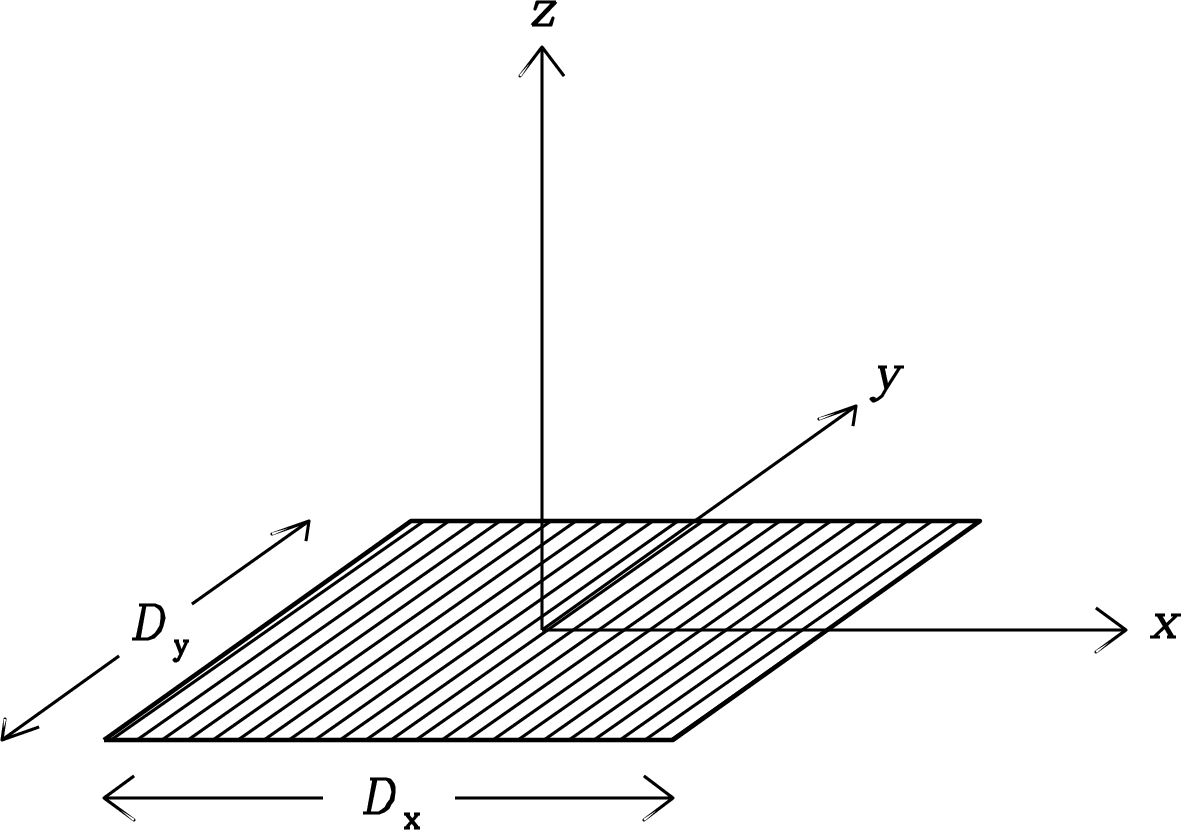
The two-dimensional counterpart of a uniformly illuminated one-dimensional aperture is a uniformly illuminated rectangular aperture with side lengths and . Dividing lengths in the aperture plane by the wavelength yields the normalized coordinates and . The direction from the origin of the plane to any distant point can be specified by and , where is the angle from the plane and is the angle from the plane (Figure 3.14). If the illumination is constant over the aperture, the integrals over and in the Fourier transform are separable and
| (3.99) |
Squaring the electric field pattern gives the relative (normalized to unity at the peak) power pattern
| (3.100) |
The absolute power gain in any direction can be calculated from the relative power pattern by invoking energy conservation:
| (3.101) | |||
| (3.102) |
Defining the temporary variable as
| (3.103) |
gives, for ,
| (3.104) |
because the value of the definite integral in square brackets is . [To prove this, simply apply Rayleigh’s theorem (Equation A.7) to the Fourier transform pair (Equation 3.77) and (Equation 3.74).] Then
| (3.105) |
Thus the peak power gain is
| (3.106) |
and the power pattern of a uniformly illuminated rectangular aperture with side lengths and is
| (3.107) | |||
| and | |||
| (3.108) | |||
when and are much smaller than 1 radian.
In general, the peak power gain of an aperture antenna is proportional to the geometric area ( in this case) of the aperture. The constant of proportionality is for a uniformly illuminated aperture and somewhat less for any other illumination pattern.
Using Equation 3.46
| (3.109) |
we find that the on-axis effective collecting area is
| (3.110) |
The peak effective area of an ideal uniformly illuminated aperture equals its geometric area, independent of wavelength. With any other illumination taper, the effective area is smaller than but proportional to the geometric area. It is useful to define the aperture efficiency as the ratio of the effective area to geometric area:
| (3.111) |
Thus for an ideal uniformly illuminated aperture and otherwise. The aperture efficiencies of most radio telescopes are %, although phased-array feeds control the illumination well enough to let ASKAP (Figure 8.6) reach %.
Large () rectangular waveguide horns are nearly uniformly illuminated unblocked apertures, so their actual gains and effective collecting areas can be calculated accurately. This makes them useful for measuring the absolute flux densities of strong sources such as Cas A and Cyg A and defining the practical flux-density scales used by radio astronomers [6].
Most apertures associated with reflectors and lenses are circular. The power pattern of a uniformly illuminated circular aperture is known as the Airy pattern.11 1 See http://www.olympusfluoview.com/java/resolution3d/index.html for an interactive plot showing how the Airy pattern behaves as a function of wavelength and aperture size.
3.3.3 Gaussian Beam Solid Angle and Beamwidth
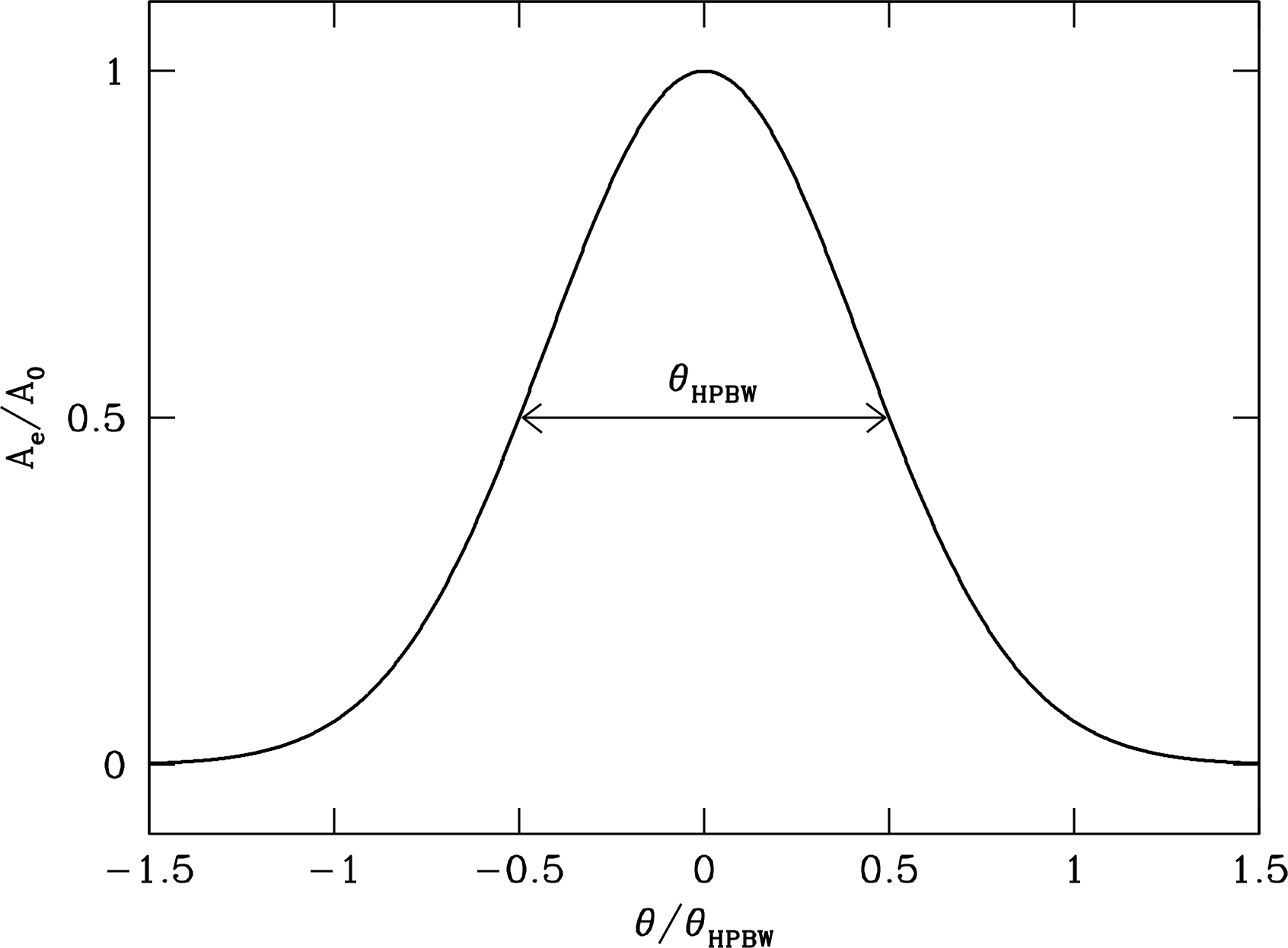
For any realistic illumination taper, the beam solid angle (Equation 3.42)
of a radio telescope is about equal to the square of the half-power beamwidth . In fact, the beams of most radio telescopes are nearly Gaussian and can be written as
| (3.112) |
where is the angle from the beam center and is a scaling factor such that when (Figure 3.15):
| (3.113) |
Thus
| (3.114) |
| (3.115) |
and
| (3.116) |
Integrating over and substituting the dummy variable yields
| (3.117) |
so the beam solid angle of a Gaussian beam is
| (3.118) |
3.3.4 Reflector Accuracy Requirements
Real radio telescopes don’t have perfectly smooth paraboloidal reflectors. Small deviations from the best-fit paraboloid may be caused by permanent manufacturing errors, changing gravitational deformations as the reflector is tilted, thermal distortions resulting from solar heating, and bending by strong winds. There will be some shortest wavelength below which these surface errors degrade the reflector performance so severely that the telescope becomes unusable. The reflector surface efficiency is defined as the power gain of the actual reflector divided by the power gain of a perfect paraboloidal reflector with the same size and illumination. The following calculation of how varies with the rms (root mean square) surface error in wavelengths is based on the classic method of Ruze [97].
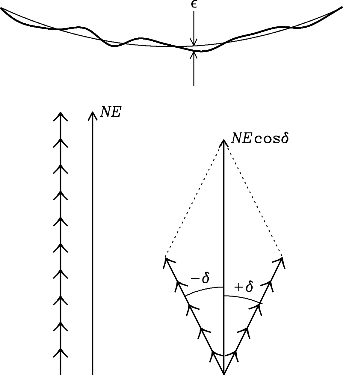
Where the actual reflector surface deviates from the best-fit paraboloid by a distance (Figure 3.16), the path length of the reflected wave will be in error by almost and the phase error (radians) of the reflected wave will be
| (3.119) |
An oversimplified example would be a bumpy surface, half covered with small bumps of height and half covered with small dips of the same depth . Then the contribution of each area element to the far (electric) field (Figure 3.16) is reduced by a factor . In the limit rad, and
| (3.120) |
so the relative power gain is
| (3.121) |
This rough estimate shows that the surface errors must be an order-of-magnitude smaller than the shortest usable wavelength, a severe requirement indeed.
A more realistic calculation makes use of the fact the most errors have roughly Gaussian amplitude distributions. Suppose that the surface errors have a Gaussian probability distribution with rms :
| (3.122) |
Then the relative field strength is obtained as the weighted sum over all possible :
| (3.123) |
Substituting turns this integral into a more familiar one, the Fourier transform of a Gaussian:
| (3.124) |
Note that the part drops out immediately because it is antisymmetric in an otherwise symmetric integral. To make this look even more familiar, let , , and . Then
| (3.125) |
Recall that the Fourier transform of is (Appendix B.4) and apply the similarity theorem (Equation A.11) to get
| (3.126) | ||||
| (3.127) | ||||
| (3.128) |
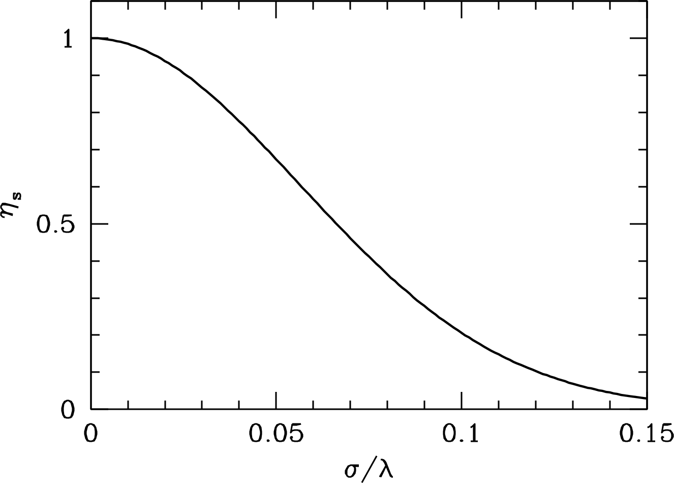
Power is proportional to so the reflector surface efficiency is simply
| (3.129) |
Equation 3.129 is often called the Ruze equation; it is plotted in Figure 3.17.
The surface efficiency is closely related to the Strehl ratio used by optical astronomers to specify the peak intensity loss caused by optical aberrations or atmospheric turbulence. The Strehl ratio is normally expressed in terms of the rms wavefront error in wavelengths , which is about twice the rms surface error in wavelengths , so Equation 3.129 implies
| (3.130) |
A traditional rule-of-thumb for the shortest wavelength at which a radio telescope works reasonably well is
| (3.131) |
because the surface efficiency at is only
| (3.132) |
and falls exponentially at shorter wavelengths. For example, the 100-m diameter GBT is intended to operate at frequencies as high as GHz, or mm. To meet this specification, the rms deviation from a perfect paraboloid must not exceed m, the thickness of two sheets of paper. The power gain of a perfect paraboloidal reflector is proportional to . If the reflector surface has a Gaussian error distribution with rms , then its gain increases as at low frequencies, reaches a maximum at
| (3.133) |
and decreases quickly at higher frequencies.
3.3.5 Pointing-Accuracy Requirements
Real radio telescopes don’t have perfectly accurate pointing. Small errors in tracking a target source reduce the gain in the source direction and contribute to the uncertainty in flux-density measurements of compact sources. Tracking errors are just as important as surface errors in limiting the short-wavelength performance of large radio telescopes.
The power patterns of most radio telescopes are nearly Gaussian near the peak. In terms of the beamwidth between half-power points , the relative gain at a point offset by angle from the beam axis is
| (3.134) |
If the one-dimensional tracking error in each coordinate (e.g., azimuth or elevation angle) has a Gaussian distribution with rms , the tracking error in two dimensions has a Rayleigh distribution
| (3.135) |
The mean squared tracking error is
| (3.136) |
The rms value of the two-dimensional tracking error is , so small tracking errors reduce the average on-source gain by the factor
| (3.137) |
More importantly, the fluctuating on-source gain caused by tracking errors contributes a fractional uncertainty22 2 http://wwwlocal.gb.nrao.edu/ptcs/ptcssn/ptcssn3.pdf.
| (3.138) |
where
| (3.139) |
to a measurement of source flux density . Thus an rms tracking error of will contribute a 10% rms flux-density uncertainty. For 5% accuracy, (or in each coordinate) is needed.
For example, we can calculate the largest tracking error in arcsec compatible with making flux-density measurements with 5% rms errors using the GBT 100-m telescope at GHz. From Equation 3.138, when . The half-power beamwidth of the GBT at GHz () is
| (3.140) |
Thus the total tracking error must be smaller than , or in azimuth and in elevation angle.
The thermal expansion coefficient of steel is about , so changing the temperature differential across the steel GBT support structure by only 1 centigrade degree could produce a pointing shift. For this reason, high-frequency observers must monitor pointing calibration sources and correct the GBT pointing every hour or so, particularly just after sunrise on sunny days. Wind gusts also degrade pointing accuracy, but they fluctuate on much shorter timescales.
3.4 Waveguides
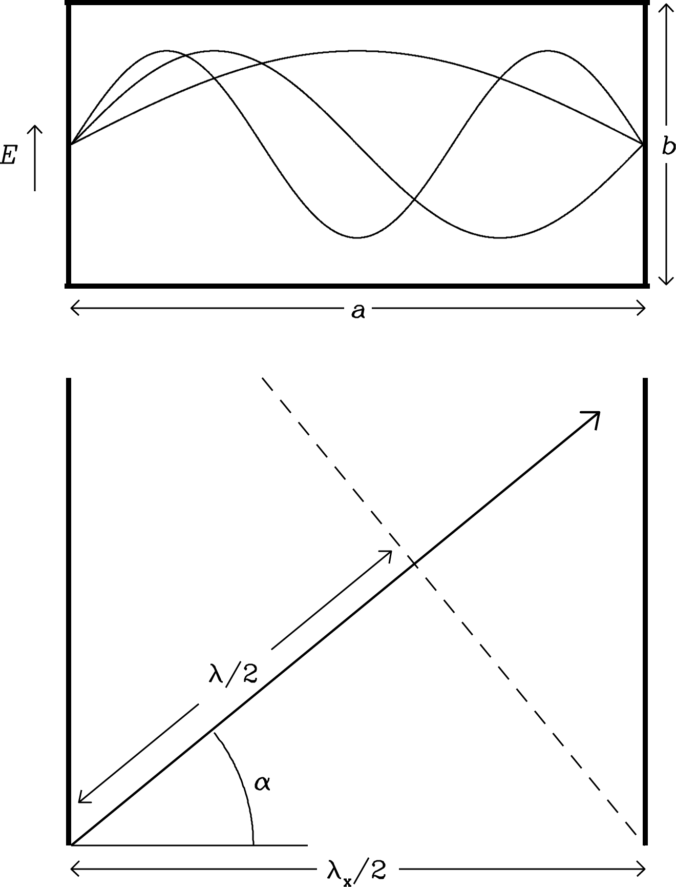
Waveguides are low-loss shielded “pipes” used to transport electromagnetic waves between antennas and receivers or between sections of a receiver. The simplest waveguide is a hollow rectangular tube with conducting walls (Figure 3.18, top) separated by distance in the horizontal () direction and in the vertical () direction. At the conducting walls, the parallel component of any electric field inside the waveguide must be zero. Three permitted distributions of the electric field strength along the horizontal axis are shown as curves in the top panel of Figure 3.18, which is similar to Figure 2.16 for standing waves in a cavity. However, only the longest-wavelength dominant mode with is normally used, and higher-order modes with are deliberately suppressed because they travel down the waveguide with different group velocities.
The bottom panel of Figure 3.18 presents the plan view of the dominant radiation mode traveling through the waveguide with a wave normal in the direction of the large arrow and a wave node () indicated by the dashed line. It is analogous to Figure 2.18 showing waves in a conducting cavity. Radiation of wavelength traveling through the waveguide in the direction indicated by the arrow must satisfy the boundary condition , where (Equation 2.66). When , .
The maximum wavelength () that can propagate () in the waveguide is the cutoff wavelength
| (3.141) |
and the corresponding minimum frequency
| (3.142) |
is called the cutoff frequency. Waveguides are extremely effective high-pass filters.
The group velocity of propagation down the waveguide is
| (3.143) |
which varies quite rapidly with frequency as approaches ( approaches 0). The waveguide phase velocity , so the guide wavelength
| (3.144) |
is somewhat greater than the free-space wavelength.
To minimize dispersion (the variation of with frequency), waveguides are rarely used at frequencies below . Higher-order modes with have frequencies and propagate with different group velocities. To suppress them, waveguides are not used for frequencies , the cutoff frequency of the mode. Practical waveguides are usually limited to frequencies . The requirement ensures that for all so , so only this TE10 (Transverse Electric field with ) mode can propagate. The TE10 mode electric field is vertically polarized and its strength is independent of .
The combination of these upper and lower frequency limits restrict most waveguide applications to octave bandwidths, and waveguides of different sizes cover different octaves. Many of the waveguide band names in use today originated as deliberately confusing code names for World War II radar bands. They and their frequency ranges are listed in Appendix F.5. For example, the standard X-band waveguide has interior dimensions , . Its cutoff wavelength is and its cutoff frequency is . Its nominal frequency range extends from to . Unfortunately, the waveguide band names are so deeply embedded in radio-astronomy jargon that radio observers cannot avoid them any more than optical astronomers can avoid “magnitudes.”
Each feed and receiver on a radio telescope covers only one waveguide band, so several feeds and receivers are needed to span the much wider useful frequency range of the telescope itself. At the VLA, the frequency range from 1 to 50 GHz is covered by eight sets of feeds and receivers in eight waveguide bands: L (1–2 GHz), S (2–4 GHz), C (4–8 GHz), X (8–12 GHz), Ku (12–18 GHz), K (18–26.5 GHz), Ka (26.5–40 GHz), and Q (40–50 GHz).
3.5 Radio Telescopes
The radio band is too wide (five decades in wavelength) to be covered effectively by a single telescope design. The surface brightnesses and angular sizes of radio sources span an even wider range, so a combination of single telescopes and aperture-synthesis interferometers are needed to detect and image them. It is not practical to build a single radio telescope that is even close to optimum for all of radio astronomy.
The ideal radio telescope should have a large collecting area to detect faint sources. The effective collecting area of any antenna averaged over all directions is (Equation 3.41)
| (3.145) |
so large peak collecting areas imply extremely directive antennas at short wavelengths. Only at long wavelengths ( m) is it feasible to construct sensitive antennas from reasonable numbers of small, nearly isotropic elements such as dipoles. Jansky’s -m “wire” antenna (Figure 1.7) is an array of phased dipoles. It produces a wide fan beam near the horizon but has a large collecting area because is so large. Directive aperture antennas are needed for adequate sensitivity at higher frequencies.
The simplest aperture antenna is a waveguide horn. Radiation incident on the opening is guided by a tapered waveguide. At the narrow end of the tapered horn is a waveguide with parallel walls, and inside this waveguide is a quarter-wave ground-plane vertical antenna that converts the electromagnetic wave into an electrical current that is sent to the receiver via a cable.
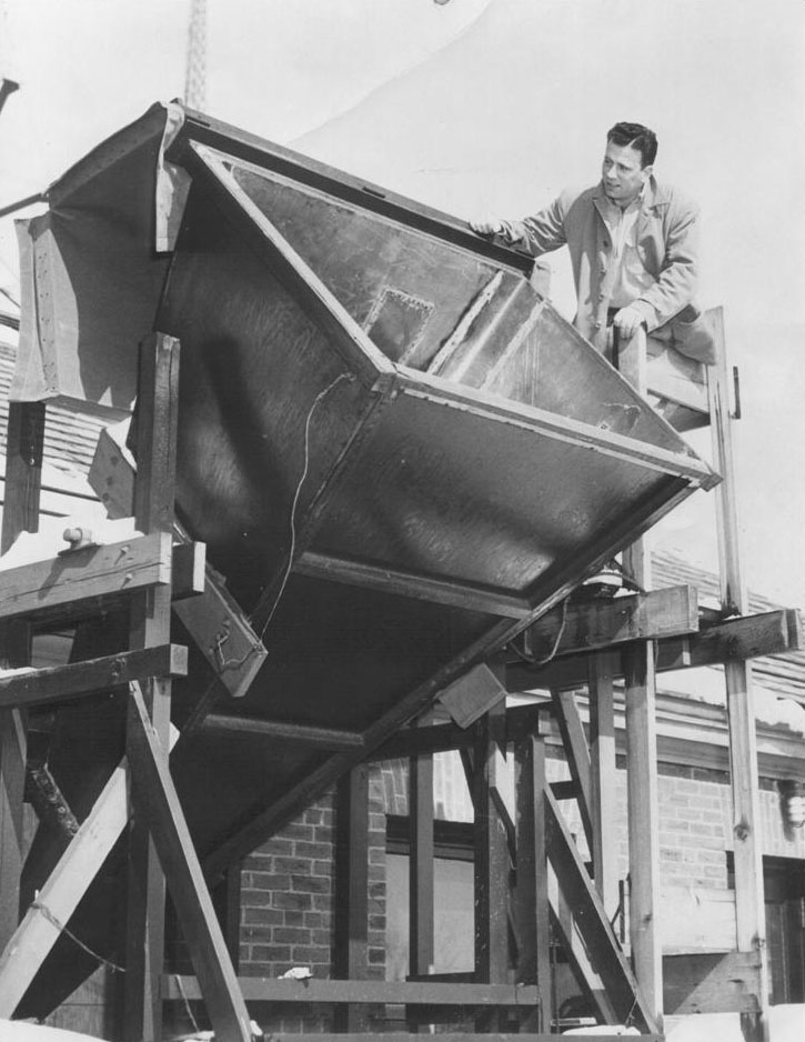
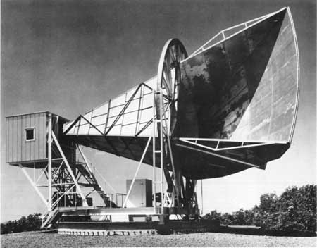
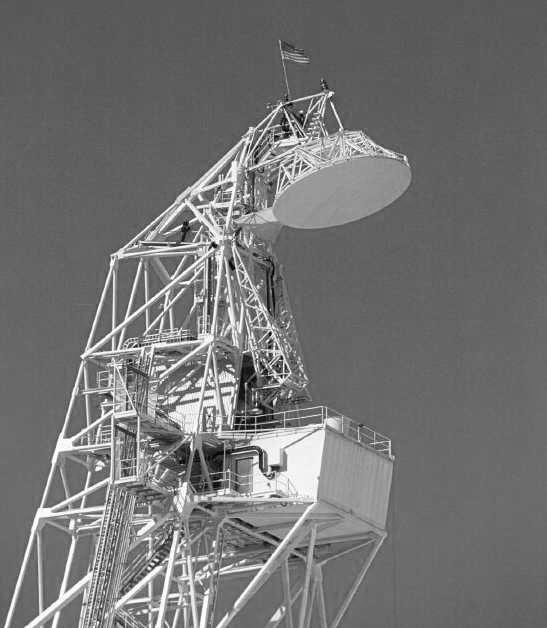
Horn antennas pick up very little ground radiation because, unlike most paraboloidal dishes, their apertures are not partially blocked by external feeds and feed-support structures, which scatter ground radiation into the receiver. This freedom from ground pickup allowed Penzias and Wilson [81] to show that the zenith antenna temperature of the Bell Labs horn (Figure 3.19) was 3.5 K higher at GHz than expected—the first detection of the cosmic microwave background radiation.
The aperture of a waveguide horn is not blocked by any feed-support structure, so it is also easier to calculate the gain of a horn antenna from first principles than to calculate the gain of a partially blocked reflecting antenna. Thus small horn antennas have been used by radio astronomers to measure the absolute flux densities of very strong sources such as Cas A. Radio astronomers observing with large dishes typically do not measure the absolute flux densities of sources, only their relative flux densities by comparison with secondary calibration sources whose flux densities relative to that of Cas A are known in advance. The painstaking process of measuring the absolute flux densities of Cas A and comparing them with the flux densities of weaker point sources suitable for calibrating observations made with large radio telescopes was described in detail by Baars et al. [6].
Most radio telescopes use circular paraboloidal reflectors to obtain large collecting areas and high angular resolution over a wide frequency range. Because the feed is on the reflector axis, the feed and legs supporting it partially block the path of radiation falling onto the reflector. This aperture blockage has a number of undesirable consequences:
-
1.
The effective collecting area is reduced because some of the incoming radiation is blocked.
-
2.
The beam pattern is degraded by increased sidelobe levels.
-
3.
Radiation from the ground that is scattered off the feed and its support structure increases the system noise.
-
4.
Radiation from the Sun and artificial sources of radio frequency interference (RFI) far from the main beam will be mixed with the desired signal.
Radio telescopes are so large that paraboloids with high ratios are impractical; typically . Thus radio “dishes” are relatively deep, as shown in Figure 3.20. Another consequence of a low ratio is a tiny field of view at the prime focus. The instantaneous imaging capability of a large single dish is severely limited by the small number of feeds that can fit into the tiny focal circle.
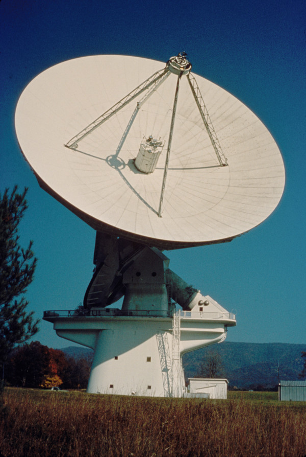
Nearly all radio telescopes have alt-az mounts consisting of a horizontal azimuth track on which the telescope turns in azimuth (the angle measured clockwise from north in the horizontal plane) and a horizontal elevation axle about which the telescope tips in altitude or elevation angle (two names for the angle above the horizon). The 140-foot telescope in Green Bank is unique among large radio telescopes in having an equatorial mount (Figure 3.20). The advantage of a equatorial mount is tracking simplicity—the declination axis is fixed and the hour-angle axis turns at a constant rate while tracking a distant celestial source. (The hour angle is the angle past the meridian, measured in hours. The meridian is the great circle passing through the north pole, south pole, and zenith.) In contrast, both the altitude and the azimuth of a celestial source change nonlinearly with time. When the 140-foot telescope was being designed, the ability of computers to perform the real-time calculations needed for an alt-az telescope to track a source accurately was in doubt. The disadvantage of a equatorial mount is mechanical—the sloped hour-angle yoke and polar axle with its huge tail bearing are very difficult to build and support.
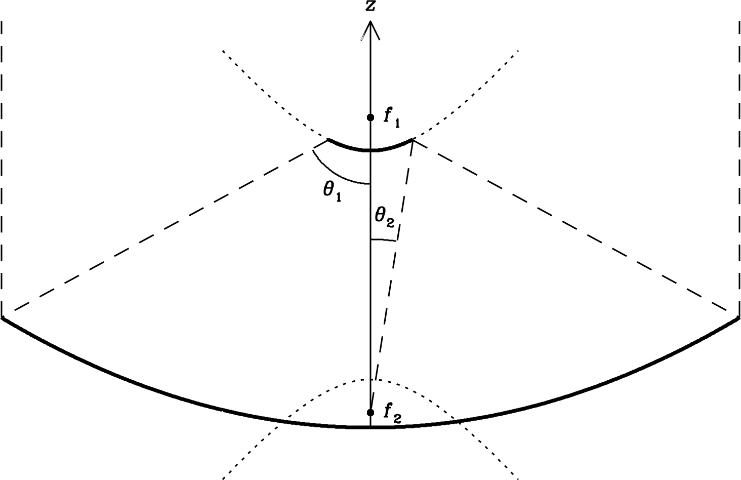
Figure 3.20 clearly shows the Cassegrain optical system of the 140-foot telescope. Radiation reflected from the main dish is reflected a second time from the convex Cassegrain subreflector located just below the focal point down to feed horns and receivers near the vertex of the paraboloid. A subreflector system has some advantages over a prime-focus system:
-
1.
The magnifying subreflector can multiply the effective ratio; values of are typical. This greatly increases the size of the focal ellipsoid. Multiple feeds can be located within the focal ellipsoid to produce multiple simultaneous beams for faster imaging.
-
2.
The subreflector is many wavelengths in diameter so it can be used to tailor the illumination taper to optimize the trade-off between high aperture efficiency and low sidelobes.
-
3.
Receivers can be located near the vertex, not the focal point, where they are easier to access.
-
4.
Feed spillover radiation is directed toward the cold sky instead of the warm ground, lowering overall system temperatures.
-
5.
The subreflector can be nutated (rocked back and forth) rapidly to switch the beam between two adjacent positions on the sky. Such differential observations in time and space can be used to remove receiver baseline drift in time and large-scale spatial fluctuations of atmospheric noise.
-
6.
The subreflector can be tilted to select one of several feeds at the secondary focus, so that the observing frequency band can be changed rapidly.
A subreflector system has some disadvantages:
-
1.
Relatively large feeds are required to produce the narrow beams needed to illuminate the subreflector, which typically subtends only a small angle as viewed from the vertex.
-
2.
Standing waves in the leaky cavity formed by the reflector and subreflector cause sinusoidal ripples with frequency period in the observed spectra of strong continuum radio sources. These ripples can be minimized by alternately defocusing the subreflector radially by and averaging the data from both subreflector positions.
-
3.
A Cassegrain subreflector blocks the prime-focus position, so prime-focus feeds cannot be used when the Cassegrain subreflector is in position.
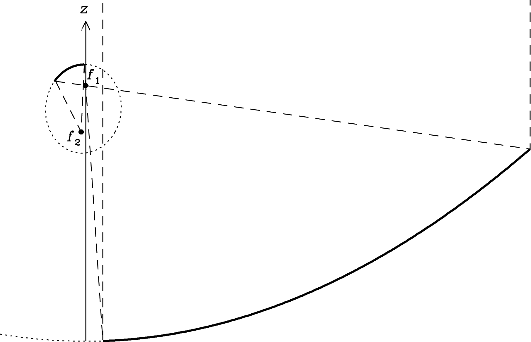
The geometry of a symmetrical radio telescope with a Cassegrain subreflector is shown in Figure 3.21. The paraboloidal shape of the primary reflector was determined by the requirement that all incoming rays parallel to the -axis travel the same distance to reach the prime focus at . Likewise, the secondary reflector shape is determined by the requirement that these rays travel the same distance to reach the secondary focus at . For a subreflector located below the prime focus, the required shape is a hyperboloid whose major axis coincides with the major axis of the paraboloid. The equation
| (3.146) |
with defines such a hyperboloid. From any point on the hyperboloid, the difference between the distance to and the distance to is . The distance between the foci is . The two free parameters and can be adjusted to set both the diameter of the subreflector as needed to intercept rays from the edge of the primary and the height of the secondary focus on the -axis. The magnification provided by the subreflector is
| (3.147) |
where is the half angle subtended by the primary viewed from and is the half angle subtended by the secondary viewed from . A small subreflector is light, easy to tilt, and reduces standing waves, but it subtends a small angle at so a feed horn several wavelengths in diameter is required to illuminate it properly.
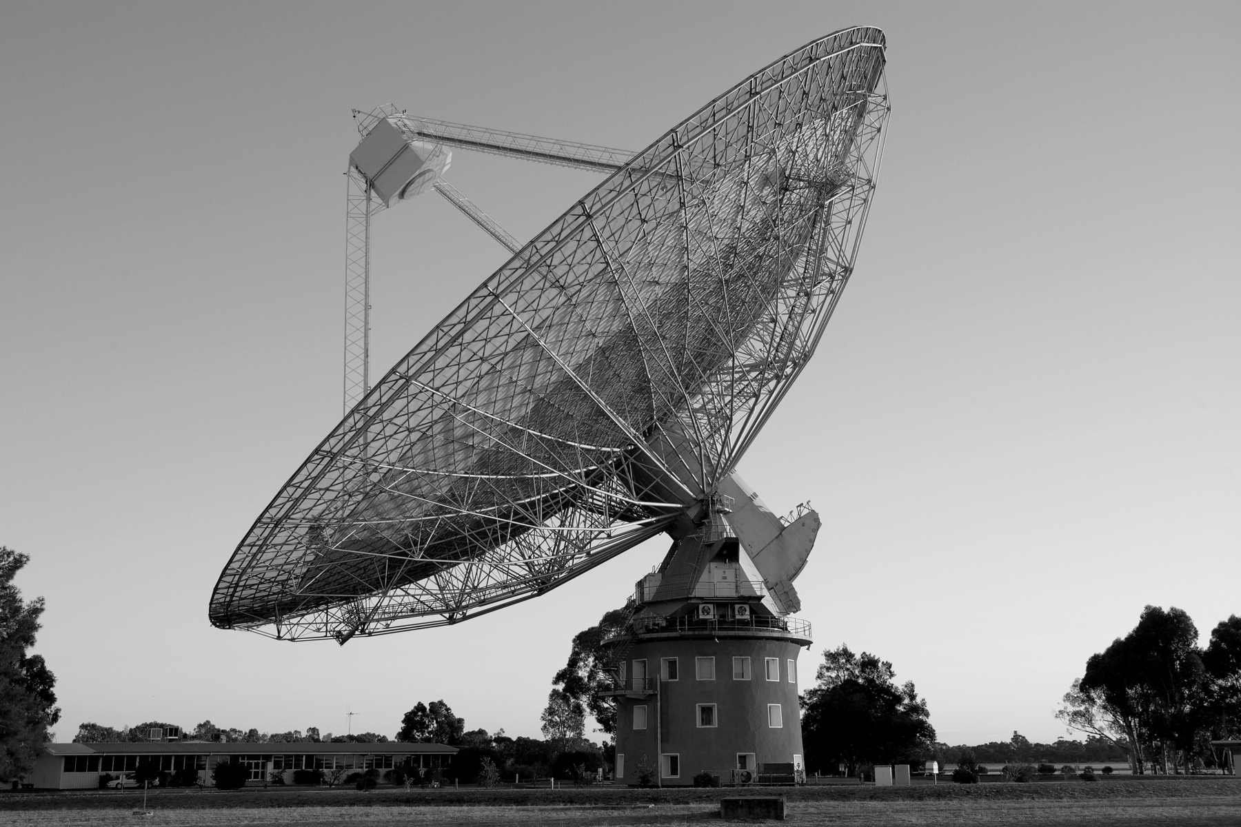
The Parkes 210-foot (since renamed to 64-m) telescope (Figure 3.22) in Australia was built about the same time as the 140-foot telescope, but its alt-az mount and centrally concentrated reflector backup structure pointed the way to the design of modern radio telescopes.
Elevation-dependent gravitational deformations degrade the short-wavelength performance of tilting reflectors. The deformations can be controlled by designing the backup structure so that the deformed surface remains paraboloidal. The deformations cause the focal point to shift slightly in elevation, but this shift can be accommodated by moving the feed slightly to track the focus. The first large homologous telescope deliberately designed to deform this way is the 100-m telescope (Figure 3.23) of the Max Planck Institut für Radioastronomie (MPIfR) near Effelsberg, Germany. Despite its huge size, its passive surface remains accurate enough to work at wavelengths as short as mm over a range of elevations.

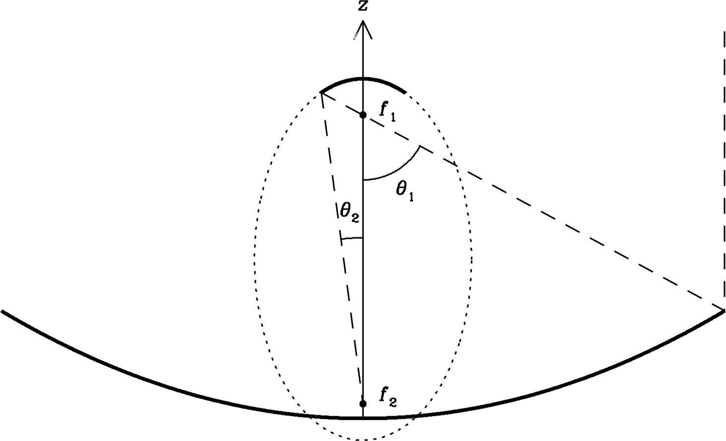
The 100-m telescope has a concave Gregorian subreflector above the prime focus. The geometry of a symmetric Gregorian system is shown in Figure 3.24. As with the Cassegrain subreflector, the Gregorian reflector shape is determined by the requirement that all parallel axial rays travel the same distance to reach the secondary focus at . For a subreflector located above the prime focus, the required shape is an ellipsoid whose major axis coincides with the major axis of the paraboloid. The equation
| (3.148) |
with defines such an ellipsoid. From any point on the ellipsoid, the sum of the distance to and the distance to is . The distance between the foci is .
The Arecibo radio telescope (Figures 8.2 and 3.25) was originally designed as a radar facility to study the ionosphere via Thomson scattering of 430 MHz ( cm) radio waves by free electrons. Thermal motions of truly free electrons would greatly Doppler broaden the bandwidth of the radar echo and lower the received signal-to-noise ratio, so a very large antenna was built for sensitivity. However, ionospheric electrons are coupled to the much heavier ions on scales larger than the ionospheric Debye length, which is only a few mm. This is much smaller than the 70 cm wavelength, so the actual bandwidth is determined by thermal motions of the much heavier ions and is lower by two orders of magnitude. Thus a far smaller dish would have sufficed! Astronomers have benefited from this oversight and use Arecibo’s huge collecting area at frequencies up to about 10 GHz for Solar-System radar (planets, moons, asteroids), pulsar studies, Hi 21-cm line observations of galaxies, and other observations that need high sensitivity.
The spherical reflector can be very large because it is does not move. A sphere is symmetric about any axis passing through its center, so the Arecibo beam can be steered by moving the feed instead of the reflector. The curved feed-support arm visible in Figure 3.25 is 300 feet long and rotates in azimuth below the fixed triangular structure. The feeds are mounted under two carriage houses that move along tracks on the bottom of the feed arm and permit tracking at zenith angles up to 20 degrees. The feed illumination spills over the edge of the fixed reflector at high zenith angles, so a large ground screen surrounds the spherical reflector to reflect the spillover onto the cold sky and keep it away from the warm and noisy ground.
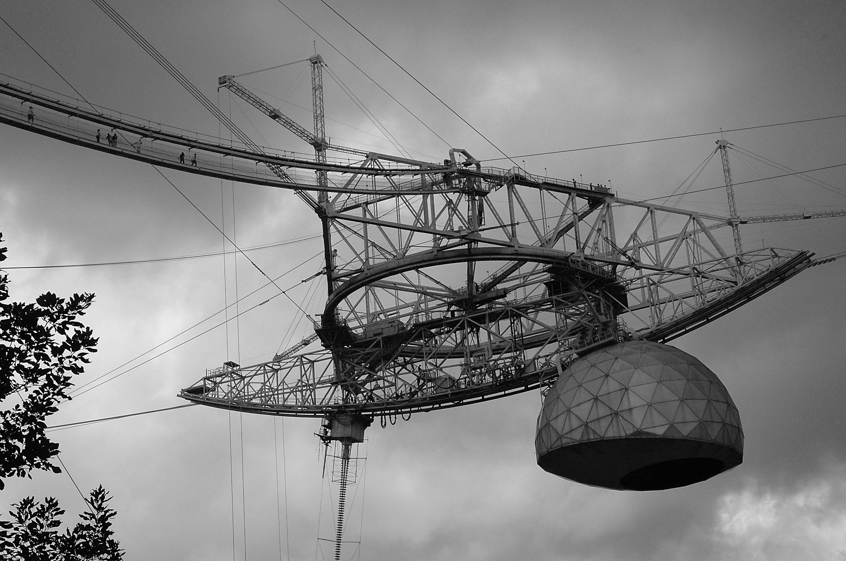
A spherical reflector focuses a distant point source onto a radial line segment, so a radial line feed (see Figure 3.25) up to 96 feet long is needed to illuminate the entire aperture efficiently from the prime focus. The line feed is a slotted waveguide tapered to control the group velocity (Equation 3.143) and phase up radiation arriving from all over the reflector. However, long slotted-waveguide line feeds are inherently narrowband, and ohmic losses in the long slotted waveguide increase the system temperature significantly at short wavelengths. The “golf ball” under the feed arm at Arecibo (Figure 3.25) houses an enormous Gregorian subreflector and a tertiary reflector that allow low-noise wideband point feeds to illuminate an ellipse about 200 m by 225 m in size on the main reflector.
The 100-m Robert C. Byrd Green Bank Telescope (GBT) (Figure 8.1) is the successor to the collapsed 300-foot telescope in Green Bank, and it incorporates a number of new design features to optimize its sensitivity and short-wavelength performance.
The actual reflector is a 110 m 100 m off-axis section of an imaginary symmetric paraboloid 208 m in diameter. Projected onto a plane normal to the beam, it is a 100-m diameter circle. Because the projected edge of the actual reflector is 4 m away from the axis of the 208-m paraboloid, the focal point does not block the aperture. The GBT enjoys the same clear-aperture benefits of waveguide horns—a very clean beam and low spillover noise—but is much larger than any practical horn antenna. The clean beam is especially valuable for suppressing radio-frequency interference (RFI) and stray radiation from very extended sources, such as Hi emission from the Galaxy.
The vertical cross section of the GBT plotted in Figure 3.26 shows how the offset Gregorian subreflector does not block any radiation falling onto the primary reflector. The Gregorian subreflector is above the prime focus at , so prime-focus operation is possible by raising a swinging boom carrying the prime-focus feeds into position below the subreflector, although this temporarily blocks the Gregorian subreflector. The huge feed-support arm is over 60 m long, the focal length of the 208-m paraboloid. The feed-support arm has a much larger cross section than the feed-support structures of symmetrical telescopes, which must be kept as thin as possible to minimize blockage. This GBT arm is very strong and can support heavy subreflectors, feeds, equipment rooms, and an elevator. At the top of the arm and above the prime focus is the concave Gregorian subreflector. This subreflector illuminates feeds emerging through the roof of a large receiver cabin attached to the feed arm a short distance below (Figure 3.27). Because these feeds are relatively close to the subreflector, even a moderately small subreflector subtends a large angle as viewed from the feeds, which can then be moderately small themselves. Most of the receivers and feeds needed to cover the frequency range can fit into the receiver cabin simultaneously and are available for use on short notice.
The main reflector is supported by a backup structure that deforms homologously to ensure good efficiency at wavelengths as short as cm. The active reflecting surface consists of approximately two thousand panels, each about 2 m on a side. The corners of individual panels are mounted on computer-controlled actuators that can move the panels up or down as needed to continuously correct the overall shape of the surface. Photogrammetry was used to measure the surface at the rigging elevation (the elevation at which the surface was originally set). The gravitational deformations at other elevation angles predicted by the finite-element computer model of the GBT are continuously removed by the actuators as the telescope moves. As a result, the rms surface error is only and the GBT has a high surface efficiency at wavelengths as short as mm.
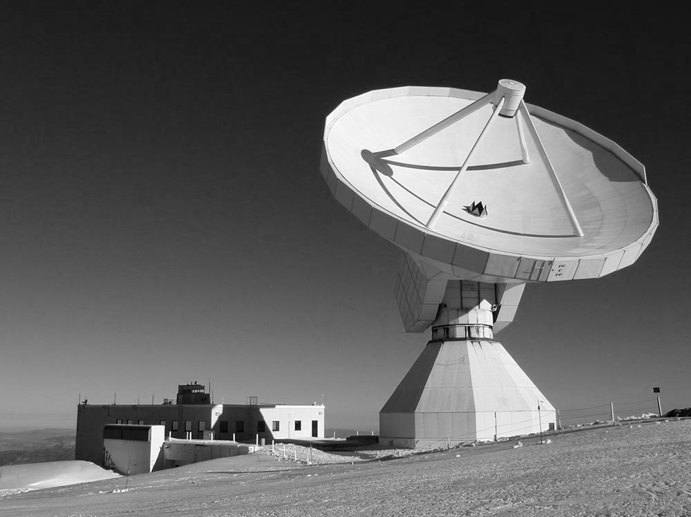
The 30-m IRAM (Institut de Radioastronomie Millimétrique) telescope (Figure 3.28) is the largest telescope operating at 3, 2, 1, and 0.8 mm. Its rms surface error is only , and its pointing accuracy is about 1 arcsec.
3.6 Radiometers
Natural radio emission from the cosmic microwave background, discrete astronomical sources, the Earth’s atmosphere, and the ground is random broadband noise that is nearly indistinguishable from the noise generated by a warm resistor (Section 2.5) or by receiver electronics. A radio receiver used to measure the average power of the noise coming from a radio telescope in a well-defined frequency range is called a radiometer. The noise voltage has a Gaussian amplitude distribution with zero mean, and it fluctuates on the very short timescales (nanoseconds) comparable with the inverse of the radiometer bandwidth . A square-law detector in the radiometer squares the input noise voltage to produce an output voltage proportional to the input noise power. Noise power is always greater than zero, and the noise from most astronomical sources is stationary, meaning that its mean power is steady when averaged over much longer timescales (seconds to hours). The Nyquist–Shannon sampling theorem (Appendix A.3) states that any function having finite bandwidth and duration can be represented by independent samples spaced in time by . By averaging a large number of independent noise samples, an ideal radiometer can determine the average noise power with a fractional uncertainty as small as and detect faint sources that increase the antenna temperature by only a tiny fraction of the total noise power. The ideal radiometer equation expresses this result in terms of the radiometer bandwidth and the averaging time. Gain variations in practical radiometers, fluctuations in atmospheric emission, and confusion by unresolved radio sources may significantly degrade the actual sensitivity compared with that predicted by the ideal radiometer equation.
3.6.1 Band-Limited Noise
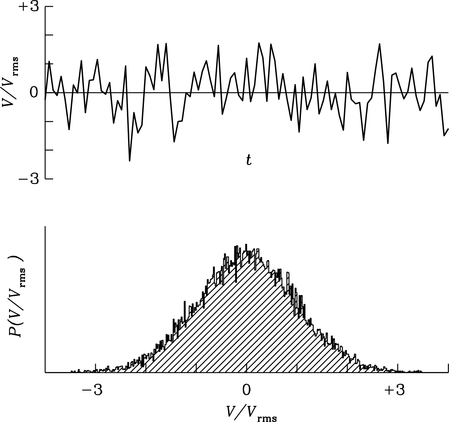
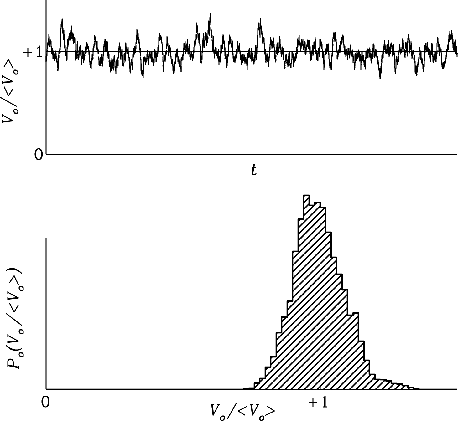
The voltage at the output of a radio telescope is the sum of noise voltages from many independent random contributions. The central limit theorem [15] states that the amplitude distribution of such noise is nearly Gaussian. Figure 3.29 (lower panel) shows the histogram of about 20,000 independent voltage samples randomly drawn from a Gaussian parent distribution having rms and mean . Figure 3.29 (upper panel) shows successive samples drawn from the Gaussian noise distribution. This sequence of voltages is representative of band-limited noise in the frequency range from 0 to during a time interval such that , e.g., noise with all frequencies up to MHz sampled every for s. This is what the band-limited noise output voltage of a radio telescope looks like.
It is convenient to describe noise power in units of temperature. The noise power per unit bandwidth generated by a resistor of temperature is in the low-frequency limit, so we can define the noise temperature of any noiselike source in terms of its power per unit bandwidth :
| (3.149) |
where joule K is Boltzmann’s constant.
The temperature equivalent to the total noise power from all sources referenced to the input of a radiometer connected to the output of a radio telescope is called the system noise temperature . It is the sum of many contributors to the antenna temperature plus the radiometer noise temperature :
| (3.150) |
There are seven antenna-temperature contributions listed explicitly in Equation 3.150:
-
1.
K is from the nearly isotropic cosmic microwave background.
- 2.
-
3.
is from the astronomical source being observed, written with a to emphasize that it is usually much smaller than the total system noise: . For example, in the GHz sky survey made with the 300-foot telescope, the system noise was K, but the faintest detected sources added only K.
-
4.
is the brightness of atmospheric emission in the telescope beam (Section 2.2.3).
-
5.
accounts for spillover radiation that the feed picks up in directions beyond the edge of the reflector, primarily from the ground.
-
6.
is the radiometer noise temperature attributable to noise generated by the radiometer itself, referenced to the radiometer input. All radiometers generate noise, and any radiometer can be represented by an equivalent circuit consisting of a noiseless radiometer whose input is connected to a resistor of temperature . Radiometer noise is usually minimized by cooling the radiometer to cryogenic temperatures. However, radiometers are not just matched resistors, so may be either lower or higher than the physical temperature of the radiometer itself.
-
7.
“” represents any other noise sources that might be important. An example is emission resulting from ohmic losses in the long slotted waveguide feed at Arecibo (Figure 3.25).
3.6.2 Radiometers
The purpose of the simplest total-power radiometer is to measure the time-averaged power of the input noise in some well-defined radio frequency (RF) range
| (3.152) |
where is the receiver bandwidth. For example, the receivers used on the 300-foot telescope to make the cm continuum survey of the northern sky had a center radio frequency Hz and a bandwidth Hz.
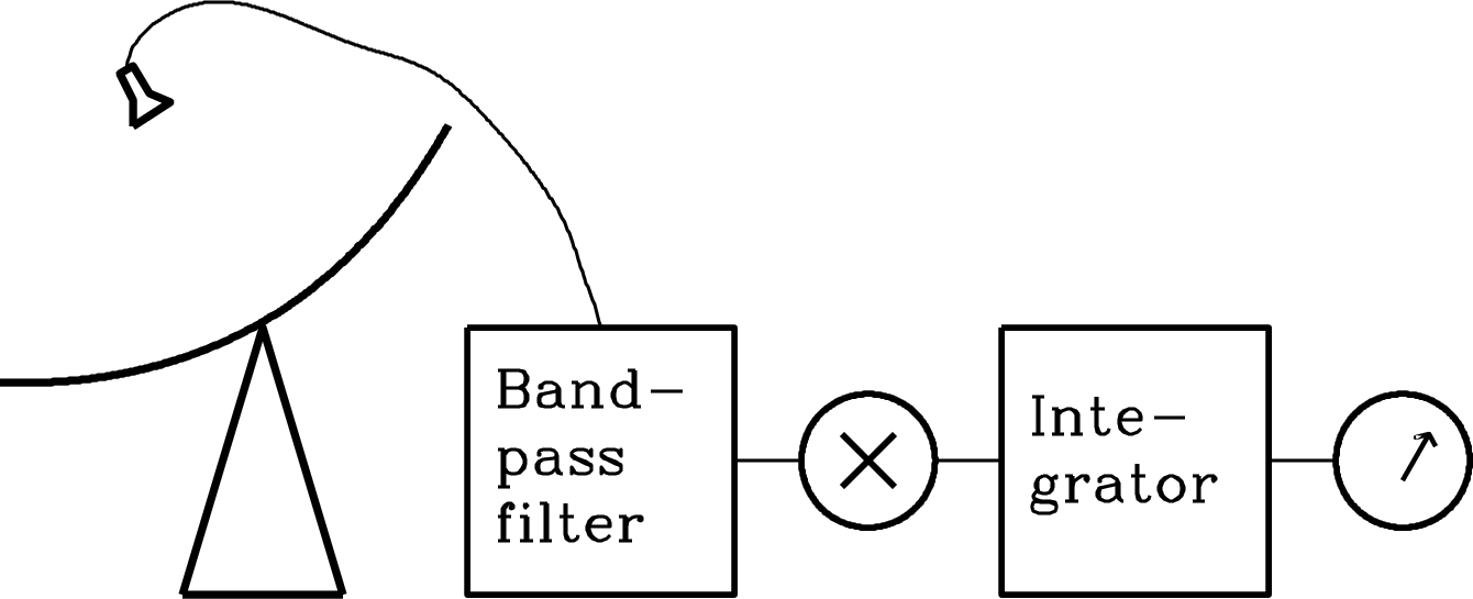
The simplest radiometer (Figure 3.30) consists of four stages in series: (1) a low-loss bandpass filter that passes input noise only in the desired frequency range; (2) a square-law detector whose output voltage is proportional to the square of its input voltage; that is, is proportional to its input power; (3) a signal averager or integrator that smooths the rapidly fluctuating detector output; and (4) a voltmeter or other device to measure and record the smoothed voltage.
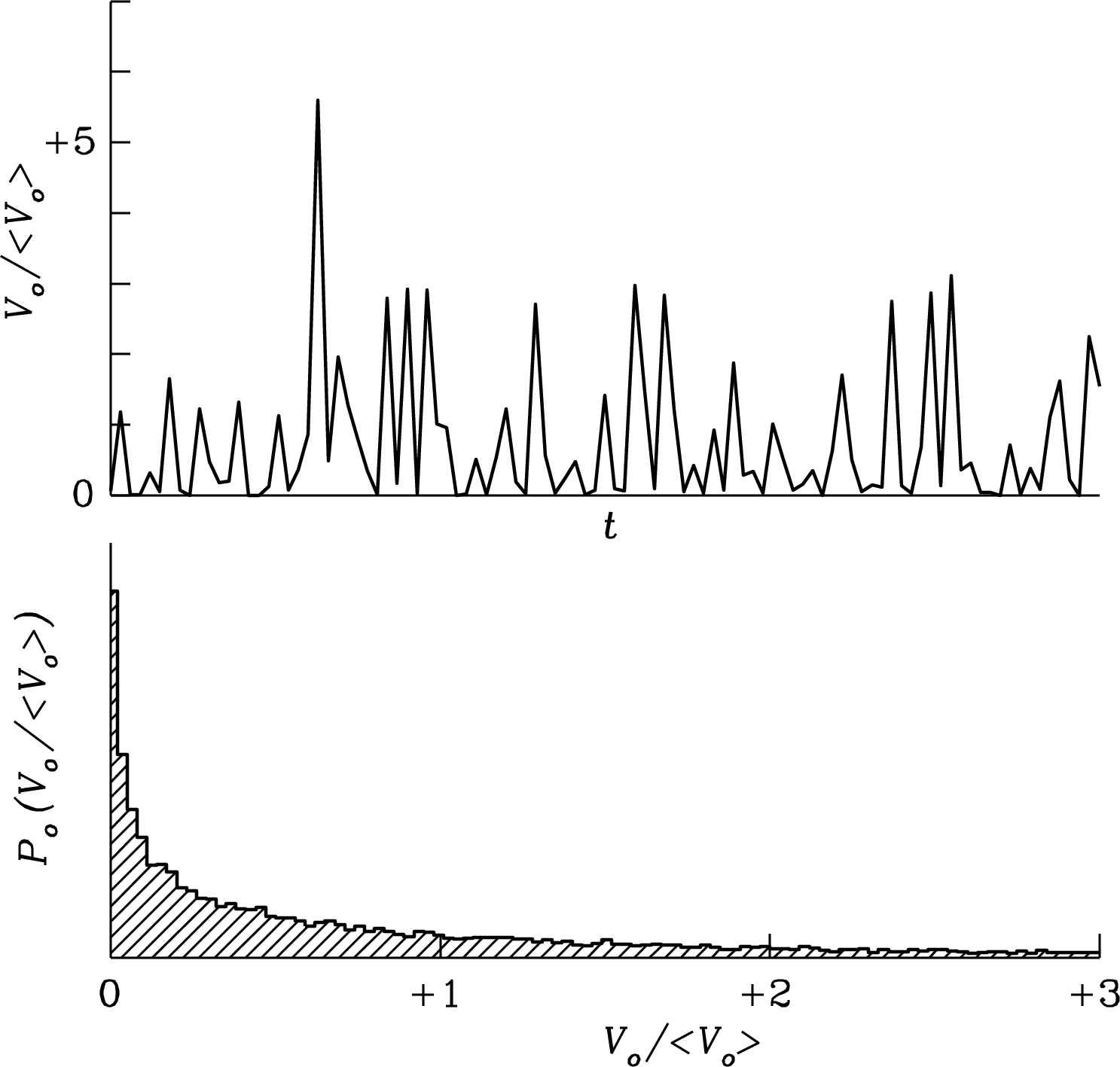
After passing through an input filter of width , the noise voltage is no longer completely random; it looks more like a sine wave of frequency whose amplitude envelope (dashed curve in Figure 3.31) varies randomly on timescales . The positive and negative envelopes are similar so long as .
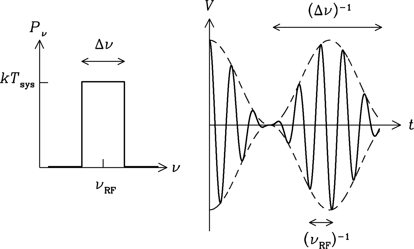
The filtered output is sent to a square-law detector whose output voltage is proportional to its input power. For a narrowband (quasi-sinusoidal) input voltage at frequency , the detector output voltage would be . This can be rewritten as , a function whose mean value is proportional to the average power of the input signal. In addition to the DC (zero-frequency) component there is an oscillating component at twice the input frequency . The detector output spectrum for a finite bandwidth and a typical waveform is shown in Figure 3.32.
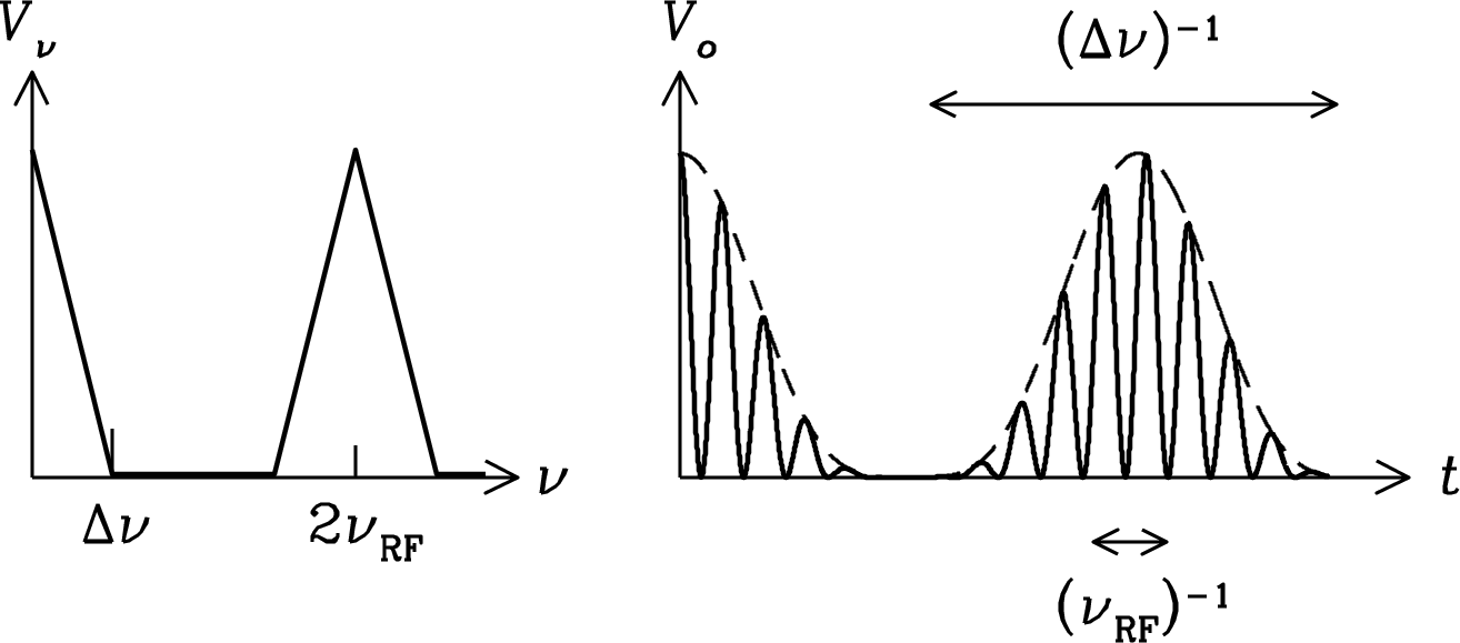
The oscillations under the envelope approach zero every . Thus the oscillating component of the detector output is centered near the frequency . The detector output also has frequency components near zero (DC) because the mean output voltage is greater than zero.
Both the rapidly varying component at frequencies near and its envelope vary on timescales that are normally much shorter than the timescales on which the average signal power varies. The unwanted rapid variations can be suppressed by taking the arithmetic mean of the detected envelope over some timescale by integrating or averaging the detector output. This integration might be done electronically by smoothing with an RC (resistance plus capacitance) filter or numerically by sampling and digitizing the detector output voltage and then computing its running mean.
Integration greatly reduces the receiver output fluctuations. In the time interval there are independent samples of the total noise power , each of which has an rms error . The rms error in the average of independent samples is reduced by the factor , so the rms receiver output fluctuation (see Appendix B.6 for a formal derivation of this result) is only
| (3.153) |
In terms of bandwidth and integration time ,
| (3.154) |
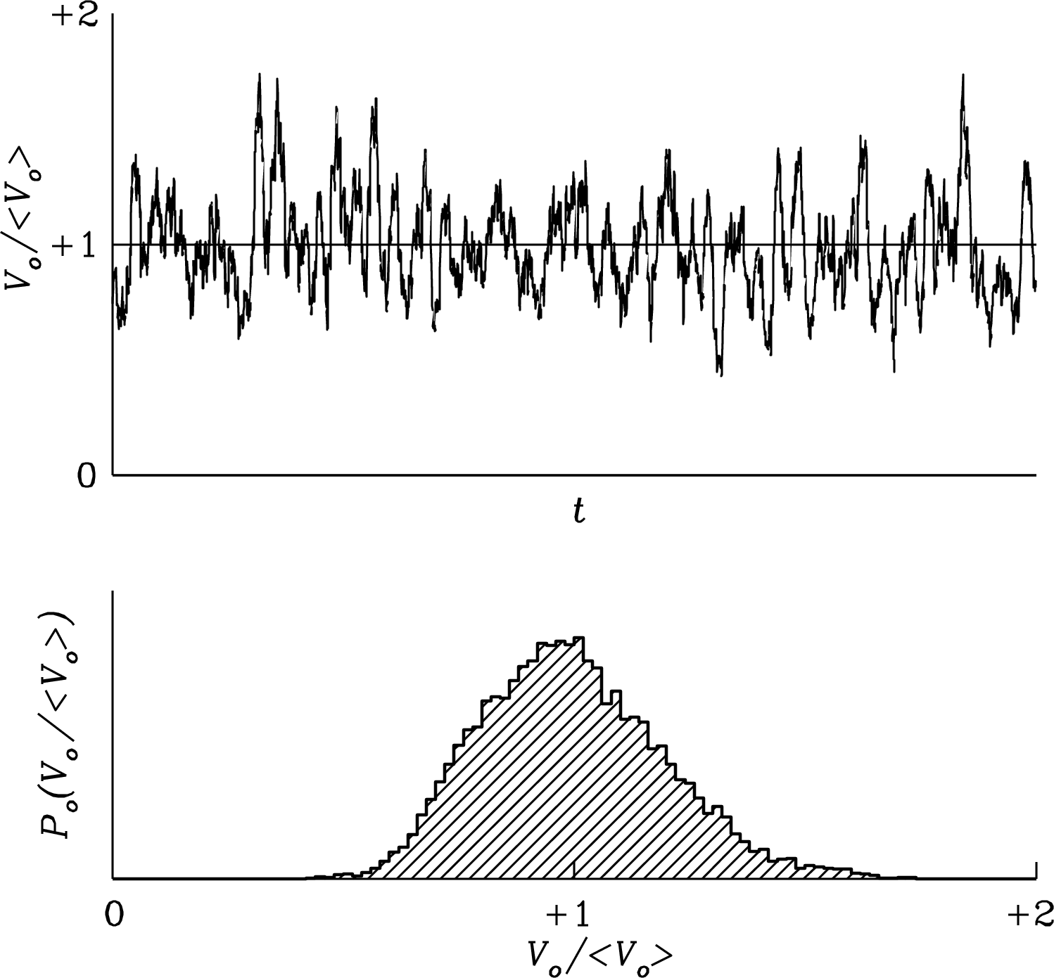
after smoothing. The central limit theorem of statistics implies that heavily smoothed () output voltages also have a nearly Gaussian amplitude distribution. This important equation is called the ideal radiometer equation for a total-power receiver. The weakest detectable signals only have to be several (typically five) times the output rms given by the radiometer equation, not several times the total system noise . The product may be quite large in practice ( is not unusual), so signals as faint as would be detectable. Figures 3.34 and 3.35 illustrate the effects of smoothing the detector output by taking running means of lengths and samples.
3.6.3 Some Caveats
The ideal radiometer equation suggests that the sensitivity of a radio observation improves as forever. In practice, systematic errors set a floor to the noise level that can be reached. Receiver gain changes, erratic fluctuations in atmospheric emission, or “confusion” by the unresolved background of continuum radio sources usually limit the sensitivity of single-dish continuum observations.
Receiver Gain and Atmospheric Fluctuations
Radiometers contain a series of amplifiers that multiply the weak input powers to milliwatt levels. The output voltage of a total-power receiver is directly proportional to the overall power gain of the receiver. If isn’t perfectly constant, the change in output voltage caused by a gain fluctuation in a practical radiometer produces a false signal whose apparent temperature
| (3.155) |
is indistinguishable from a comparable change caused by noise in an ideal radiometer. Receiver gain fluctuations and noise fluctuations are independent random processes, so their variances (the variance is the square of the rms) add, and the total receiver output fluctuation becomes
| (3.156) | ||||
| (3.157) |
The practical total-power radiometer equation is thus
| (3.158) |
Clearly, radiometer gain fluctuations will degrade the sensitivity of an observation unless
| (3.159) |
For example, the 5 GHz receiver used to make the sky survey with the 300-foot telescope had Hz and s, so the fractional gain fluctuations on timescales up to a few seconds (the time to scan one baseline length) had to satisfy
| (3.160) |
This is difficult to achieve in practice. Gain fluctuations typically have “” power spectra, where is the postdetection frequency, so they are larger on longer timescales and increasing eventually results in a higher output noise level. The gain stability of a receiver is often specified by the “ knee” frequency , the postdetection frequency at which . Integrations longer than will likely increase the receiver output fluctuations. Depending on the stability and bandwidth of the radiometer, .
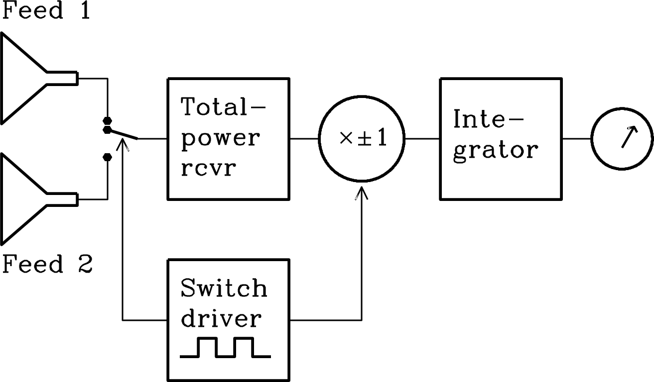
Fluctuations in atmospheric emission also add to the noise in the output of a simple total-power receiver. Water vapor is the main culprit because it is not well mixed in the atmosphere, and noise from water-vapor fluctuations can be a significant problem at frequencies of GHz and up.
One way to minimize the effects of fluctuations in both receiver gain and atmospheric emission is to make a differential measurement by comparing signals from two adjacent feeds. The method of switching rapidly between beams or loads is called Dicke switching after Robert Dicke, its inventor. Figure 3.36 shows the block diagram of a beam-switching Dicke radiometer. If the system temperatures are and in the two positions of the switch, then the receiver output is proportional to and the effect of gain fluctuations is only
| (3.161) |
Likewise, the atmospheric emission in two nearly overlapping beams through the troposphere is nearly the same, so most of the tropospheric fluctuations cancel out. The main drawback with Dicke switching is that the receiver output fluctuations, relative to the source signal in a single beam, are doubled because the source signal is being received only half the time while the noise power is present all the time. The ideal radiometer equation for a Dicke switching receiver is
| (3.162) |
Confusion
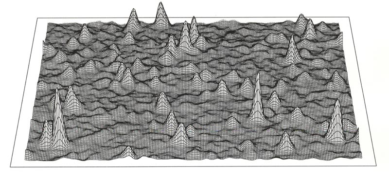
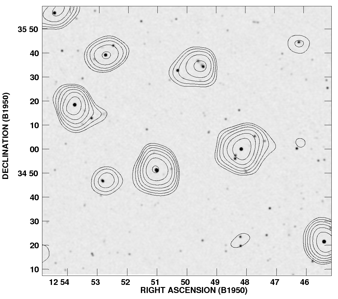
Single-dish radio telescopes have large collecting areas but relatively broad beams at long wavelengths. Nearly all discrete continuum sources are extragalactic and extremely distant, so they are distributed randomly and isotropically on the sky. The sky-brightness fluctuations caused by numerous faint sources in every telescope beam are called confusion, and confusion usually limits the sensitivity of single-dish continuum observations at frequencies below . Figure 3.37 is a profile plot of confusion fluctuations in a low-resolution image. Figure 3.38 shows contours from a portion of that low-resolution image superimposed on an overlapping high-resolution gray-scale image.
Although the amplitude distribution of confusion is distinctly non-Gaussian, the “rms” confusion calculated by ignoring the long positive tail is a widely quoted. At cm wavelengths, the rms confusion in a Gaussian telescope beam with FHWM is
| (3.163) |
Individual sources fainter than the confusion limit cannot be detected reliably, no matter how low the receiver noise. Most continuum observations of faint sources at frequencies below are made with interferometers instead of single dishes because interferometers can synthesize much smaller beamwidths and hence have significantly lower confusion limits.
Confusion by steady continuum sources has a much smaller effect on observations of spectral lines or rapidly varying sources such as pulsars.
3.6.4 Superheterodyne Receivers
Few actual radiometers are as simple as those described above. Nearly all practical radiometers are superheterodyne receivers (Figure 3.39), in which the RF amplifier is followed by a mixer that multiplies the RF signal by a sine wave of frequency generated by a local oscillator (LO). The product of two sine waves contains the sum and difference frequency components,
| (3.164) |
so the mixer acts as a frequency shifter. For example, if and , the mixer output frequency, called the intermediate frequency (IF), will be .
The advantages of superheterodyne receivers include
-
1.
shifting the signals to lower frequencies where they are easier to amplify, transmit over long distances, filter, and digitize;
-
2.
tunability over a wide range of ;
-
3.
tuning by adjusting only the local oscillator frequency so that
-
4.
the IF amplifier and back-end devices such as multichannel filter banks or digital spectrometers can all operate over fixed frequency ranges.
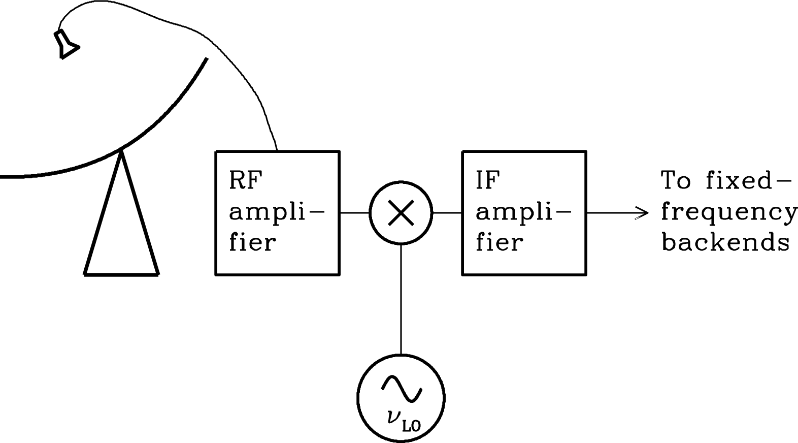
3.6.5 Spectrometers
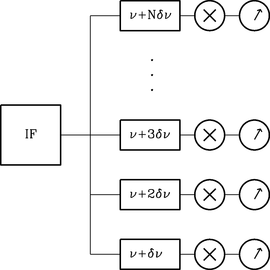
The simplest superheterodyne radiometer measures the total power in its normally broad IF passband of width . A spectrometer is a backend that divides that passband into adjacent narrow frequency ranges of width and simultaneously measures the power in all channels to quickly locate and resolve spectral features such as atomic and molecular lines (Section 7.1).
The most straightforward spectrometer is a filter bank of narrowband analog filters connected in parallel and with center frequencies uniformly spaced by (Figure 3.40). Each channel acts as a separate IF and has its own detector. However, the channel gains, bandpasses, and detector responses of an analog filter bank must be very closely matched and stable to yield smooth spectral baselines, so analog filter banks with more than channels are difficult to build and tune. Analog filter banks are also inflexible because their channel bandwidths and numbers cannot be changed easily. Flexible spectrometers with or even frequency channels require digital signal processing (DSP) techniques.
For many years, most digital spectrometers were autocorrelation spectrometers using the Wiener–Khinchin theorem (Equation A.18) to compute power spectra from digitally sampled time series (see Appendix A.3) of the band-limited IF output. A sampled copy of a portion of the input radio signal is delayed by a series of progressively longer time delays, the delayed signals are multiplied with the original signal, and their products are integrated. This series of operations is an autocorrelation (Appendix A.7). If the digital samples contain only one or two bits (two or three levels) each, autocorrelation can be performed in hardware and often in a single chip, with relatively simple digital logic. These autocorrelation functions (ACFs) can be integrated to build up signal-to-noise and then finally converted into a power spectrum via a discrete Fourier transform (usually an FFT; see Appendix A.2) of the ACF via the Wiener–Khinchin theorem. Autocorrelation spectrometers allow the integration of very deep (i.e., long-duration) spectra using relatively simple digital hardware and without computing many “costly” FFTs directly on incoming Nyquist-sampled data; only one FFT is computed at the very end of the integration. Similar techniques, but using cross-correlation of the signals from different antennas, are often used to calculate spectra from radio interferometers.
With the continuing improvements in the speeds and capabilities of DSP systems, spectra are increasingly being computed directly via FFTs of a Nyquist-sampled band. The Fourier amplitudes are squared to make power spectra, and the power spectra are accumulated for deep spectral integrations. Such systems are known as Fourier transform spectrometers, and the FFTs can be computed in a variety of ways. Many recent spectrometers use Field Programmable Gate Arrays (FPGAs) to compute the FFTs, integrate, and compute polarization products, all on a single chip. Other hybrid designs use FPGAs to divide the band into coarse channels and pass those effectively Nyquist-sampled subbands off to CPUs, other FPGAs, or Graphical Processing Units (GPUs) for further processing, such as coherent dedispersion and folding of pulsar data in a pulsar back-end, or much finer frequency resolution and perhaps even active interference removal for high-sensitivity spectroscopy applications. The new VErsatile GBT Astronomical Spectrometer (VEGAS) is a hybrid Fourier transform spectrometer. The capabilities of such systems, especially given the fidelity provided by sampling with eight or more bits precision, is making them the new standard back-end technology for radio astronomy.
3.6.6 Measuring Radiometer Noise
The radiometer itself usually contributes significantly to the total system noise temperature . Any radiometer can be modeled by an equivalent circuit consisting of an ideal noiseless radiometer plus an input matched load resistor at temperature , where is called the radiometer input noise temperature.
The simplest way to measure is to connect a matched “hot” load resistor whose physical temperature is to the radiometer input and record the detector output voltage , and then replace it with a “cold” load whose physical temperature is and record the output voltage . Often the hot load is just a resistor at room temperature and the cold load is a resistor immersed in liquid nitrogen at its boiling temperature .
For each measurement, the square-law detector output voltage is proportional to the total input noise power generated by the actual load plus the imaginary resistor whose temperature is . In the low-frequency Nyquist approximation , so
| (3.165) | ||||
| (3.166) |
where is the bandwidth and is the overall gain of the radiometer. Both and cancel out in the factor defined by
| (3.167) |
so they do not have to be measured. Equation 3.167 can be solved for the radiometer noise temperature
| (3.168) |
This technique for measuring is called the -factor method.
Communications engineers often specify the radiometer noise factor defined by
| (3.169) |
where the standard temperature defined as is close to room temperature. The numerator in Equation 3.169 is proportional to the detected output voltage of the radiometer connected to an ambient-temperature load and the denominator is the output of a noiseless radiometer connected to an ambient-temperature load. In terms of , the radiometer noise temperature is
| (3.170) |
The related radiometer noise figure NF used by many commercial manufacturers of amplifiers and radiometers is just the noise factor expressed in dB:
| (3.171) |
3.7 Interferometers
Every practical single-dish radio telescope (Section 3.5) has relatively low angular resolution and pointing accuracy, small field-of-view, and limited sensitivity. The largest fully steerable dish has diameter m and its angular resolution is diffraction limited to radians, so impossibly large diameters would be needed to achieve sub-arcsecond resolution at radio wavelengths. Pointing and source-tracking accuracy is also a problem for a large single dish. The telescope beam should be able to follow a radio source on the sky within for reasonably accurate photometry or imaging. The accuracy with which the actual beam direction during an observation can be recovered by later data analysis determines the accuracy with which the sky position of a radio source can be measured. Gravitational sagging, telescope deformations caused by differential solar heating, and torques caused by wind gusts combine to limit the mechanical tracking and pointing accuracies of the best radio telescopes to arcsec. Most optical telescopes can make high-resolution images covering large areas of sky rapidly because their large fields-of-view cover millions or billions of pixels. In contrast, most single-dish radio telescopes have only one or several beams. The geometric area of a single dish is just , while the geometric area of an interferometer with dishes can be arbitrarily large. The continuum sensitivity of a single dish is strongly limited by confusion at frequencies below about 10 GHz.
Aperture-synthesis interferometers comprising moderately small dishes have mitigated these and many other practical problems associated with single dishes, such as vulnerability to fluctuations in atmospheric emission and receiver gain, radio-frequency interference, and pointing shifts caused by atmospheric refraction. For example, the Westerbork Synthesis Radio Telescope (Figure 8.3) consists of , telescopes on east–west baselines up to in length. Its total collecting area is that of a single dish with diameter m. It has the high angular resolution of a diffraction-limited telescope 3 km in diameter. It has the large instantaneous field-of-view of a 25-m telescope, so it can image pixels at once with only one receiver on each telescope. It can measure positions of radio sources with subarcsecond accuracy despite the much larger source-tracking errors of the individual telescopes.
Historically, the total bandwidths and numbers of simultaneous frequency channels of aperture-synthesis interferometers with many dishes were lower than those of single dishes. Recent advances in correlator electronics and computing have largely overcome these practical limitations, so new or updated interferometers such as ALMA (Figure 8.5) and the JVLA (Figure 8.4) are playing an increasingly dominant role in observational radio astronomy. The primary uses of single dishes today are
-
(a)
observing pulsars, which are time variable so they are easy to separate from confusion by time-independent continuum sources;
-
(b)
spectroscopic observations of extended low-brightness sources, again largely immune to confusion;
-
(c)
complementing interferometers by providing “zero-spacing” data on very extended sources or by serving as elements of very long baseline arrays.
3.7.1 The Two-Element Quasi-Monochromatic Interferometer
The simplest radio interferometer is a pair of radio telescopes whose voltage outputs are correlated (multiplied and averaged), and even the most elaborate interferometers with antennas, often called elements, can be treated as independent two-element interferometers.
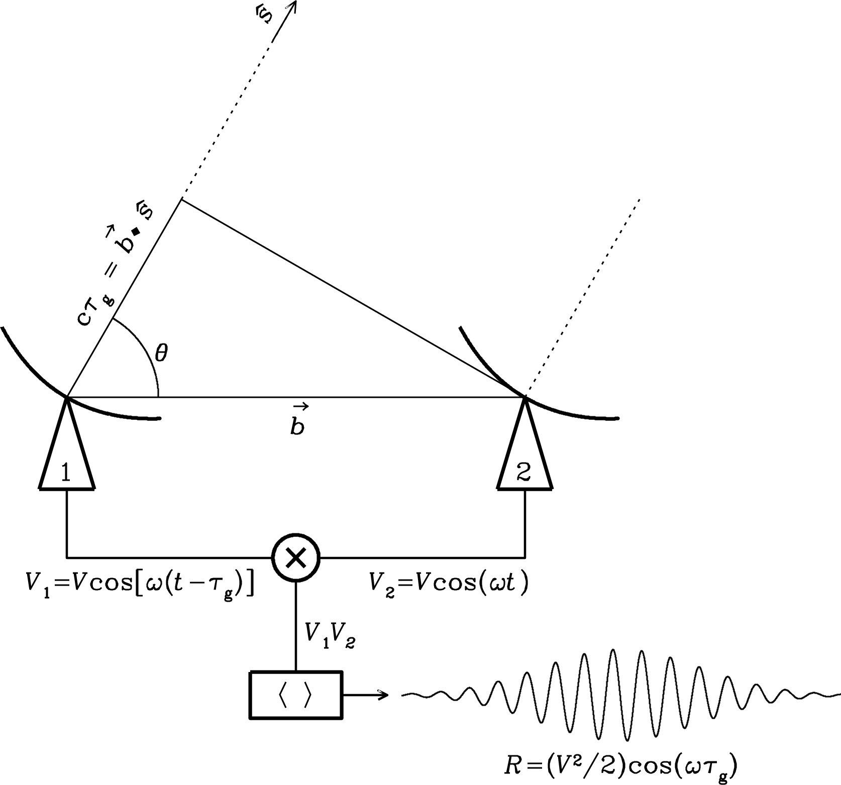
Figure 3.41 shows two identical dishes separated by the baseline vector of length that points from antenna 1 to antenna 2. Both dishes point in the same direction specified by the unit vector , and is the angle between and . Plane waves from a distant point source in this direction must travel an extra distance to reach antenna 1, so the output of antenna 1 is the same as that of antenna 2, but it lags in time by the geometric delay
| (3.172) |
For simplicity, we first consider a quasi-monochromatic interferometer, one that responds only to radiation in a very narrow band centered on frequency . Then the output voltages of antennas 1 and 2 at time can be written as
| (3.173) |
These output voltages are amplified versions of the antenna input voltages; they have not passed through square-law detectors. Instead, a correlator multiplies these two voltages to yield the product
| (3.174) |
that follows directly from the trigonometric identity . The correlator also takes a time average long enough () to remove the high-frequency term from the correlator response (output voltage) and keep only the slowly varying term
| (3.175) |
The voltages and are proportional to the electric field produced by the source multiplied by the voltage gains of the two antennas and receivers. Thus the correlator output amplitude is proportional to the flux density of the point source multiplied by , where and are the effective collecting areas of the two antennas.
Notice that the time-averaged response of a multiplying interferometer is zero. There is no DC output, so fluctuations in receiver gain do not act on the whole system temperature as for a total-power observation with a single dish (Equation 3.155). Uncorrelated noise power from very extended radio sources such as the cosmic microwave background and the atmosphere over the telescopes, also averages to zero in the correlator response. Short interference pulses with duration are also suppressed because each pulse does not reach both telescopes simultaneously. Likewise, a multiplying radio interferometer differs from a classical adding interferometer, such as the optical Michelson interferometer, that adds the uncorrelated noise power contributions.
The correlator output voltage varies sinusoidally as the Earth’s rotation changes the source direction relative to the baseline vector. These sinusoids are called fringes, and the fringe phase
| (3.176) |
depends on as follows:
| (3.177) | ||||
| (3.178) |
The fringe period corresponds to an angular shift . The fringe phase is an exquisitely sensitive measure of source position if the projected baseline is many wavelengths long. Note that fringe phase and hence measured source position is not affected by small tracking errors of the individual telescopes. It depends on time, and times can be measured by clocks with much higher accuracy than angles (ratios of lengths of moving telescope parts) can be measured by rulers. Also, an interferometer whose baseline is horizontal is not affected by the plane-parallel component of atmospheric refraction, which delays the signals reaching both telescopes equally. Consequently, interferometers can determine the positions of compact radio sources with unmatched accuracy, as shown in Figure 1.6. Absolute positions with errors as small as arcsec and differential positions with errors down to arcsec rad have frequently been measured.
If the individual antennas comprising an interferometer were isotropic, the interferometer point-source response would be a sinusoid spanning the sky. Such an interferometer is sensitive to only one Fourier component of the sky brightness distribution: the component with angular period . The response of a two-element interferometer with directive antennas is that sinusoid multiplied by the product of the voltage patterns of the individual antennas. Normally the two antennas are identical, so this product is the power pattern of the individual antennas and is called the primary beam of the interferometer. The primary beam is usually a Gaussian much wider than a fringe period, as indicated in Figure 3.41. The convolution theorem (Equation A.15) states that the Fourier transform of the product of two functions is the convolution of their Fourier transforms, so the interferometer with directive antennas responds to a finite range of angular frequencies centered on (). Because the antenna diameters must be smaller than the baseline (else the antennas would overlap), the angular frequency response cannot extend to zero and the interferometer cannot detect an isotropic source—the bulk of the 3 K cosmic microwave background for example. The missing short spacings () can be provided by a single-dish telescope with diameter . Thus the = 100 m GBT can fill in the missing baselines that the = 25 m VLA dishes cannot obtain.
Improving the instantaneous point-source response pattern of an interferometer requires more Fourier components; that is, more baselines. An interferometer with antennas contains pairs of antennas, each of which is a two-element interferometer, so the instantaneous synthesized beam (the point-source response obtained by averaging the outputs of all of the two-element interferometers) rapidly approaches a Gaussian as increases. The instantaneous point-source responses of a two-element interferometer with projected baseline length , a three-element interferometer with three baselines (projected lengths , , and ), and a four-element interferometer with six baselines (projected lengths , , , , , and ) are shown in Figure 3.42.
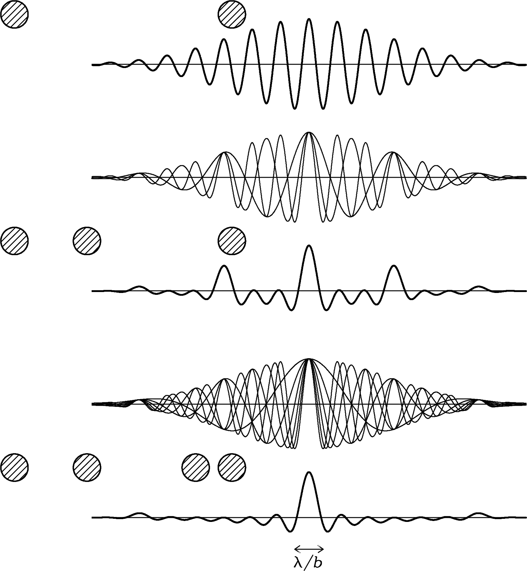
Most radio sources are stationary; that is, their brightness distributions do not change significantly on the timescales of astronomical observations. For stationary sources, a two-element interferometer with movable antennas could make observations to duplicate one observation with an -element interferometer.
3.7.2 Slightly Extended Sources and the Complex Correlator
The response of the quasi-monochromatic two-element interferometer with a “cosine” correlator (Figure 3.41 and Equation 3.175) to a spatially incoherent slightly extended (much smaller than the primary beamwidth) source with sky brightness distribution near frequency is obtained by treating the extended source as the sum of independent point sources:
| (3.179) |
Notice that the even cosine function in this response is sensitive only to the even (inversion-symmetric) part of an arbitrary source brightness distribution, which can be written as the sum of even and odd (antisymmetric) parts: . To detect the odd part we need a “sine” correlator whose output is odd, . This can be implemented by a second correlator that follows a phase delay inserted into the output of one antenna because . Then
| (3.180) |
The combination of cosine and sine correlators is called a complex correlator because it is mathematically convenient to treat the cosines and sines as complex exponentials using Euler’s formula (Appendix B.3)
| (3.181) |
The complex visibility is defined by
| (3.182) |
which can be written in the form
| (3.183) |
where
| (3.184) |
is the visibility amplitude and
| (3.185) |
is the visibility phase. The response to an extended source with brightness distribution of the two-element quasi-monochromatic interferometer with a complex correlator is the complex visibility
| (3.186) |
3.7.3 Effects of Finite Bandwidths and Averaging Times
Equation 3.186 for quasi-monochromatic interferometers may be generalized to interferometers with finite bandwidths and integration times, which are necessary for high sensitivity. In the small but finite frequency range centered on frequency , Equation 3.186 becomes
| (3.187) | ||||
| (3.188) |
If the source brightness and the response of the interferometer are nearly constant over , the integral over frequency is just the Fourier transform of a rectangle function, so
| (3.189) |
For a finite bandwidth and delay , the fringe amplitude is attenuated by the factor . This attenuation can be eliminated in any one direction called the delay center or the phase reference position by introducing a compensating delay in the signal path of the “leading” antenna, as shown in Figure 3.43. As the Earth turns, must be continuously adjusted to track within a tolerance . This is usually done with digital electronics.
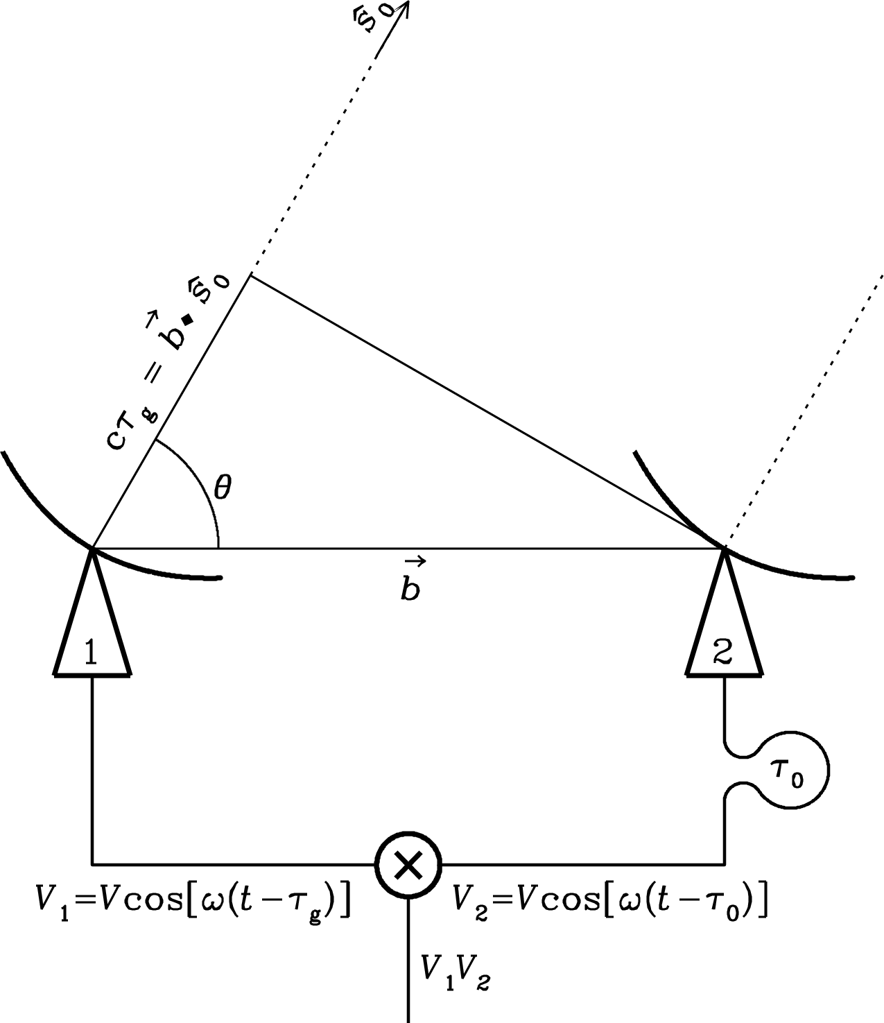
The geometric delay varies with direction, so delay compensation can be exact in only one direction. The angular radius of the usable field-of-view is determined by the variation of with offset from the direction . Because , . Requiring
| (3.190) |
implies
| (3.191) |
Substituting and using for the synthesized beamwidth, we get the requirement
| (3.192) |
At larger angular offsets from the phase reference position, bandwidth smearing will radially broaden the synthesized beam by convolving it with a rectangle of angular width .
Satisfactory wide-field images can be made with a larger total bandwidth only by dividing that bandwidth into a number of narrower frequency channels each satisfying Equation 3.192. For example, the synthesized beamwidth of the VLA “B” configuration (maximum baseline length ) at () is . To image out to an angular radius equal to the half-power radius of the VLA primary beam requires channel bandwidths
| (3.193) |
Likewise, the correlator averaging time must be kept short enough that the Earth’s rotation will not move the source position in the frame of the interferometer by as much as the synthesized beamwidth . For example, if the delay is set to track the north celestial pole, a source away from the north pole will appear to move at an angular rate , where is the Earth’s sidereal rotation period. Excessive correlator averaging times will cause time smearing that tangentially broadens the synthesized beam. To minimize time smearing in an image of angular radius , we require
| (3.194) |
Continuing with the previous example, to image out to an angular radius when requires averaging times short enough that
| (3.195) |
3.7.4 Earth-Rotation Aperture Synthesis
The Earth’s rotation varies the projected baseline coverage of an interferometer whose elements are fixed on the ground. In particular, all baselines of an interferometer whose baselines are confined to an east–west line will remain in a single plane perpendicular to the Earth’s north–south rotation axis as the Earth turns daily. Confining all baselines to two dimensions has the computational advantage that the brightness distribution of a source is simply the two-dimensional Fourier transform of the measured visibilities.
Figure 3.44 illustrates Earth-rotation aperture synthesis by an east–west two-element interferometer at latitude as viewed from a source at declination . Let be the east–west component of the projected baseline in wavelengths and be the north–south component of the projected baseline in wavelengths.
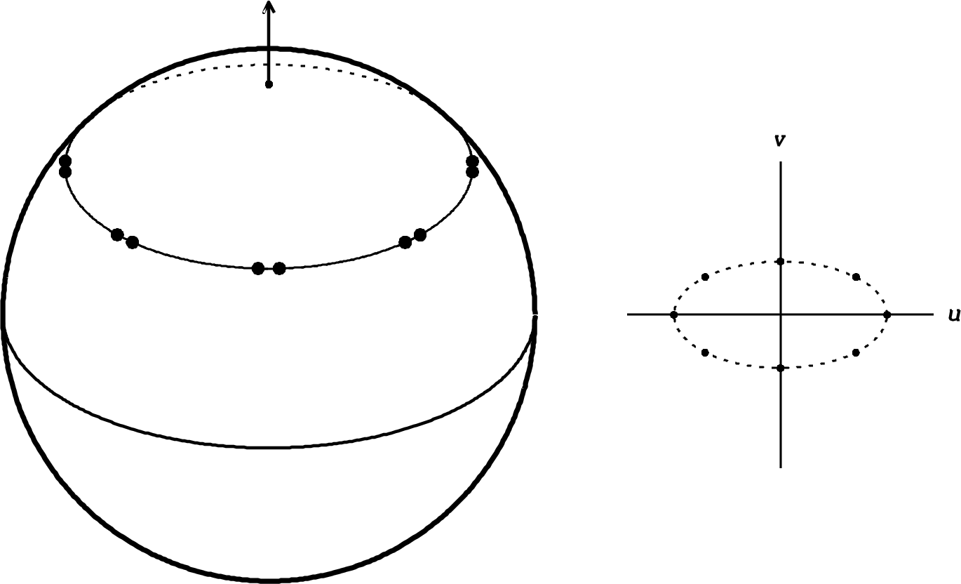
During the 12-hour period centered on source transit, the interferometer traces out a complete ellipse on the plane. The maximum value of equals the actual antenna separation in wavelengths, and the maximum value of is smaller by the projection factor , where is the source declination. If the interferometer has more than two elements, or if the spacing of the two elements is changed daily, the coverage will become a number of concentric ellipses having the same shape. Thus the synthesized beam obtained by east–west Earth-rotation aperture synthesis can approach an elliptical Gaussian. The synthesized beamwidth is radians east–west and radians in the north–south direction. The synthesized beam is circular for a source near the celestial pole, but the north–south beamwidth is very large for a source near the celestial equator.
3.7.5 Interferometers in Three Dimensions
The VLA (Very Large Array) shown in Figure 8.4 is Y-shaped and is instantaneously a nearly coplanar two-dimensional array of 27 25-m telescopes on the high Plains of San Augustin in New Mexico. It baselines are not confined to an east–west line but it is nearly coplanar, so “snapshot” observations much shorter than a sidereal day can be treated as two dimensional. On longer timescales, Earth rotation causes the VLA baselines to fill a three-dimensional volume. The north–south baselines allow imaging with a nearly circular synthesized beam even near the celestial equator. Figure 8.4 shows the “D” configuration spanning about 1 km. The telescopes can be moved along railroad tracks to form the “C”, “B”, and “A” configurations spanning 3.4, 11, and 36 km, respectively for higher angular resolution. The VLA recently underwent a major upgrade to become the JVLA (the “J” stands for “Jansky”), with new wideband receivers completely covering the frequency range 1 to 50 GHz and a far more powerful and versatile correlator. It is up to an order of magnitude more sensitive than the original narrow-band VLA.
The coordinate system used to describe any baseline vector in three dimensions is shown in Figure 3.45. The -axis is in the reference direction usually chosen to contain the target radio source. The - and -axes point east and north in the plane normal to the -axis. , , and are the components of , the baseline vector in wavelength units. An arbitrary unit vector has components as drawn, where . The components are called direction cosines.
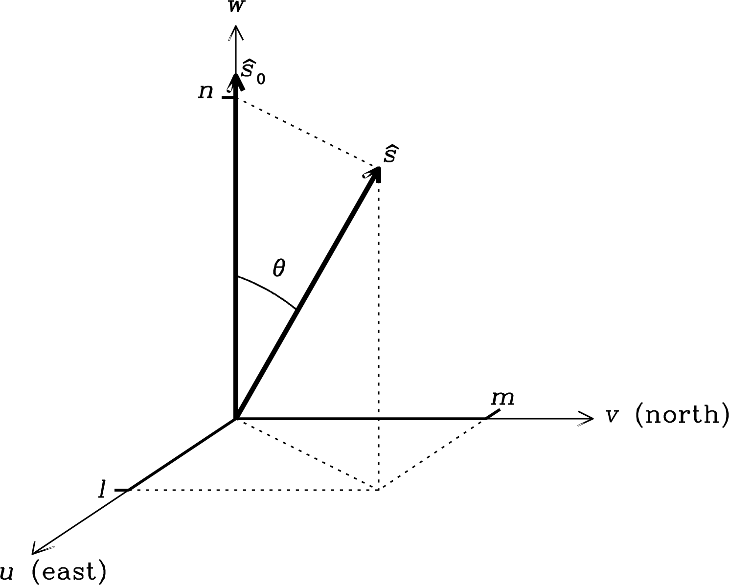
Because
| (3.196) |
the three-dimensional generalization of Equation 3.186 is
| (3.197) |
This is not a three-dimensional Fourier transform.
However, if , Equation 3.197 becomes a two-dimensional Fourier transform, which can be inverted to give the source brightness distribution in terms of the measured visibilities:
| (3.198) |
That is the case for an Earth-rotation aperture synthesis by an east–west interferometer if we choose to coincide with the Earth’s rotation axis, in which case , where is the declination of the reference position.
For any interferometer, if we consider only directions close to , then and
| (3.199) |
The factor can be kept close to unity by keeping ; that is, by imaging only a small field of view whose radius is . For example, radians is sufficiently small for an interferometer baseline wavelengths long. Then
| (3.200) |
A field wider than can be imaged with two-dimensional Fourier transforms by breaking it up into smaller facets, much like a fly’s eye, and merging the facets to make the final image.
3.7.6 Sensitivity
The point-source sensitivity of a two-element interferometer can be derived from the radiometer equation for a total-power receiver on a single antenna because a square-law detector is equivalent to a correlator multiplying two identical input voltages supplied by one antenna. Consider an interferometer with two identical elements, each of which also has a square-law detector, observing a point source. The correlator multiplies the voltages from the two antennas, while each square-law detector multiplies the voltage from one antenna by itself, so the correlated/detected output voltages of the interferometer and each single dish are equal in strength. Thus the effective collecting area of the two-element interferometer equals the effective collecting area of each element. However, the noise voltages from the two interferometer elements are almost completely uncorrelated (only the point source contributes correlated noise), while the noise voltages going into the square-law detectors are completely correlated (identical). The correlator output voltage distribution before smoothing is shown in Figure 3.46, and Figure 3.47 shows the correlator output voltage distribution after smoothing over samples. In the limit where the antenna temperature contributed by the point source is much smaller than the system noise , the correlator output noise is lower than the square-law detector noise from each antenna. For an unpolarized point source of flux-density , then , so for a single antenna,
| (3.201) |
and for a two-element interferometer,
| (3.202) |
The point-source sensitivity of a two-element interferometer is therefore times better than the sensitivity of each antenna, but times worse than that of a single dish whose area is that of two antennas. The reason the two-element interferometer is less sensitive than a single dish having the same total collecting area is that the information contained in the two independent square-law detector outputs has been discarded. Together they have times the sensitivity of a single dish. Combined with the independent correlator output, the total sensitivity is twice the sensitivity of a single dish, or exactly the sensitivity of a single dish whose area equals the total area of the two-element interferometer.
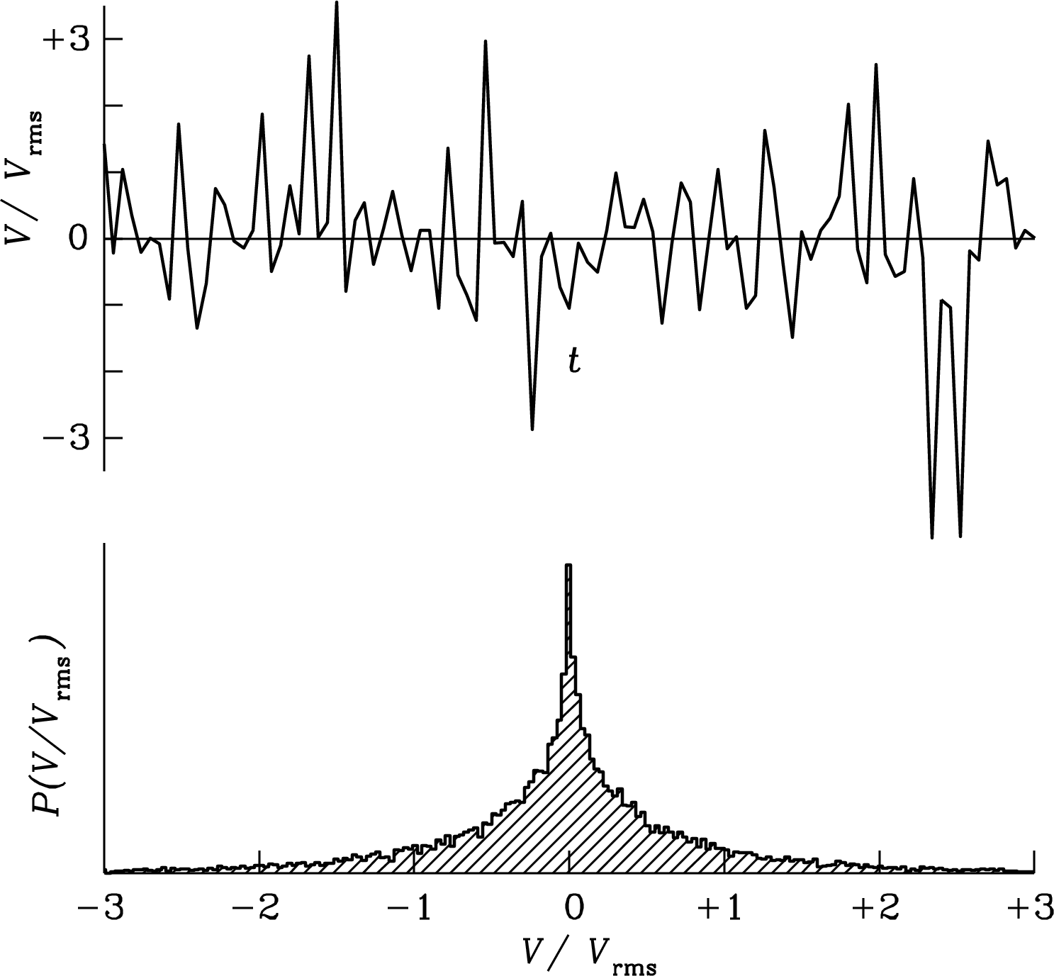
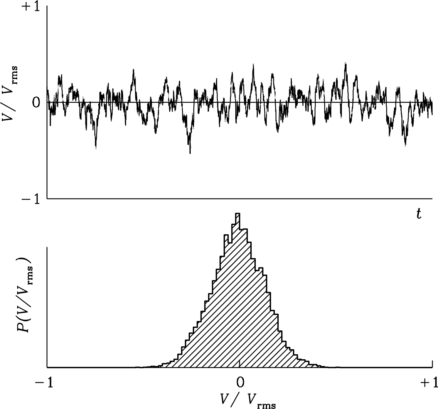
An interferometer with dishes contains independent two-element interferometers. So long as the signal from each dish can be amplified coherently before it is split up to be multiplied by the signals from the other antennas, its point-source rms noise is
| (3.203) |
In the limit of large , and the point-source sensitivity of an interferometer approaches that of a single antenna whose area equals the total effective area of the interferometer antennas. For example, the VLA with dishes each m in diameter has the point-source sensitivity of a single dish whose diameter is . Had the square-law detector outputs been used as well, the point-source sensitivity of the -element interferometer would be exactly the same as the sensitivity of a single dish having the same total collecting area.
Practical interferometers are slightly less sensitive than this because their correlators use digital multipliers that sample and quantize the input voltage, not perfect analog multipliers. For example, a digital multiplier that samples at twice the Nyquist rate with three quantization levels () is only 0.89 times as sensitive as a perfect analog multiplier. The chapter “Digital Signal Processing” in Thompson et al. [107] covers this and other consequences of quantization in detail.
Although the point-source sensitivity of an interferometer is comparable with the point-source sensitivity of a single dish having the same total area, beware that the brightness sensitivity of an interferometer is much worse because the synthesized beam solid angle of an interferometer is much smaller than the beam solid angle of a single dish of the same total effective area. The angular resolution of an interferometer with maximum baseline is and the angular resolution of the single dish with diameter is , so the beam solid angle of the interferometer is smaller by a factor . This is roughly the area filling factor of the interferometer, defined as the ratio of the area covered by all of the antennas to the area spanned by the interferometer array. For example, the VLA in its “B” configuration has a filling factor . A high-resolution interferometer cannot detect a source of low surface brightness, no matter how high its total flux density.
The intensity axis of any astronomical image has dimensions of spectral brightness or specific intensity (e.g., units of Jy per beam solid angle or MJy sr or K), not flux density (e.g., Jy). The point-source rms in Equation 3.203 corresponds to image flux density per beam solid angle, e.g., Jy beam. Published radio images usually have intensity axes in units of Jy beam because the flux density of a point source equals its brightness in those units and because is independent of beam solid angle. However, a proper spectral brightness depends only on the source. The “spectral brightness” specified in Jy beam has the dimensions of spectral brightness, but beware that this is not a proper spectral brightness because it depends on the synthesized beam solid angle and not just on the radio source. Infrared astronomers frequently specify image intensity in MJy sr, which is a proper brightness. The brightness temperature is a convenient proper brightness for radio images. The rms brightness-temperature sensitivity of an image made with beam solid angle follows directly from and the Rayleigh–Jeans approximation:
| (3.204) |
Most interferometer images are restored with Gaussian beams. The beam solid angle (Equation 3.34) of a Gaussian beam with HPBW is (Equation 3.118)
so
| (3.205) |
For example, all of the 1.4 GHz NRAO VLA Sky Survey (NVSS) images have rms noise and were restored with a circular Gaussian beam whose half-power beamwidth is . Consequently, NVSS rms brightness temperature noise is
This is good enough to detect () normal spiral galaxies with median at 1.4 GHz. Beware that a high-resolution (low ) image with a good point-source sensitivity (low ) may still have a poor brightness-temperature sensitivity (high ).