Chapter 4 Free–Free Radiation
4.1 Thermal and Nonthermal Emission
Larmor’s formula (Equation 2.143)
| (4.1) |
states that electromagnetic radiation with power is produced by accelerating (or decelerating; hence the German name bremsstrahlung meaning “braking radiation”) an electrical charge . Free charged particles can be accelerated by electrostatic or magnetic forces, gravitational acceleration being negligible by comparison. Electrostatic bremsstrahlung is the subject of this chapter, and its magnetic counterpart magnetobremsstrahlung or “magnetic braking radiation” (e.g., synchrotron radiation) is covered in Chapter 5.
Thermal emission is produced by a source whose emitting particles are in local thermodynamic equilibrium (LTE) (Section 2.2.2); otherwise nonthermal emission is produced. Most astronomical sources of electrostatic bremsstrahlung are thermal because the radiating electrons have the Maxwellian velocity distribution (Appendix B.8) of particles in LTE. The relativistic electrons in most astronomical sources of magnetobremsstrahlung have power-law energy distributions and hence are not in LTE, so synchrotron sources are often called nonthermal sources. However, electrostatic and magnetic bremsstrahlung are not synonymous with thermal and nonthermal radiation, respectively. For example, electrons with a relativistic Maxwellian energy distribution are in LTE and can emit thermal synchrotron radiation. Remember also that a thermal source does not have a blackbody spectrum if the source opacity is small and the emission coefficient depends on frequency.
4.2 Hii Regions
The electrostatic force is so much stronger than gravity that free charges in interstellar gas quickly rearrange themselves so that the negative charges of free electrons in an ionized cloud neutralize the positive charges of ions on all scales larger than the Debye length (Equation 4.46). As an electron (charge statcoulomb) passes by an ion (charge for an atom with electrons removed), the Coulomb force (Equation 2.134) causes an acceleration of magnitude
| (4.2) |
where g is the electron mass and is the distance between the electron and the ion. The resulting emission is called free–free radiation because the electron is free both before and after the interaction; it is not captured by the ion. If the ionized interstellar cloud is reasonably dense, the electrons and ions interact often enough that they quickly come into LTE at some common temperature, so free–free radiation is usually thermal emission.
Interstellar gas is primarily hydrogen and helium, plus trace amounts of heavier elements such as carbon, nitrogen, oxygen, neon, silicon, and iron. Astronomers call all of these heavier elements metals, meaning elements that readily form positive ions, even though most are not metallic in the usual sense of being solid, malleable, ductile, and electrically conducting solids at room temperature. Much of the interstellar hydrogen is in the form of neutral atoms (called Hi in astronomical terminology) or diatomic molecules (H), but some is ionized. The singly ionized hydrogen atom H is referred to as Hii by astronomers, doubly ionized oxygen O is called Oiii, triply ionized carbon C is called Civ, etc.
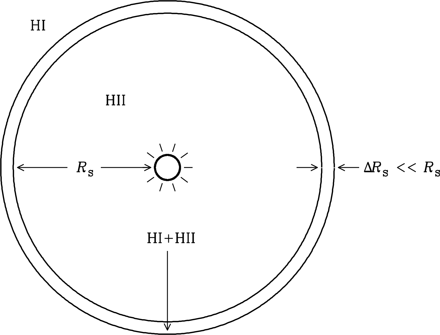
In 1939 the astronomer Bengt Strömgren realized that the interstellar medium can be divided into distinct regions in which hydrogen is either (1) mostly atomic or molecular, with nearly all of the hydrogen atoms in the ground electronic state or (2) almost completely ionized. Furthermore, the boundaries separating these Hi and Hii regions are very thin. Sometimes the Hii regions surrounding stars are called Strömgren spheres (Figure 4.1) after his early theoretical models. What is the microscopic physical basis for this picture?
A hydrogen atom in the ground state has the smallest and most tightly bound electronic orbit around the nuclear proton that is consistent with a stationary electronic wave function. (See Section 7.2.1 and Figure 7.1 to review the Bohr model of hydrogen atoms.) The permitted electronic energy levels are characterized by their principal quantum numbers where corresponds to the ground state. Although quantum mechanics forbids an electron in the ground state from radiating according to the classical Larmor formula, it permits radiative decay from higher levels and Larmor’s equation fairly accurately predicts the radiative lifetimes of excited hydrogen atoms. The orbital radius of an electron in the th energy level is , where cm is called the Bohr radius. Applying Larmor’s equation shows that the radiative lifetime is proportional to and hence to . Thus the (incorrect) classical result s for radiation from the ground state can be scaled to estimate the radiative lifetimes of excited states. For example, the approximate radiative lifetime of the state would be s, in reasonable agreement with the accurate quantum-mechanical result s. Excited hydrogen atoms spontaneously decay very quickly to the ground state by emitting radiation so, at any instant, almost all neutral atoms are in the ground state.
Hydrogen atoms in the ground state can be ionized by photons with energy eV (1 electron Volt erg). Such energetic photons have frequencies higher than the Rydberg frequency (Equation 7.11) and wavelengths shorter than Å m, a far-ultraviolet (UV) wavelength. These Lyman continuum photons are produced in significant numbers by the Wien tail of blackbody radiation from stars hotter than K. The rate at which a star with spectral luminosity produces photons that can ionize hydrogen atoms in the ground state is
| (4.3) |
If a star emits Lyman continuum photons per second, it will photoionize hydrogen atoms with number density throughout some volume surrounding the star. The helium mixed with the hydrogen can often be ignored because its ionization potential is so high, eV, that only exceptionally hot stars can ionize significant amounts of helium.
The absorption cross section of a neutral hydrogen atom to photons with energies just above 13.6 eV is large enough, , that each ionizing photon is absorbed and produces a new ion shortly after it passes from the ionized Strömgren sphere into the surrounding Hi region. The thickness of the partially ionized shell surrounding a Strömgren sphere (Figure 4.1) is
| (4.4) |
For example, if the neutral hydrogen density is , then
| (4.5) |
Light travels cm per hour, so an ionizing photon typically survives only about an hour in such an Hi cloud before being absorbed.
Once ionized from Hi into free protons (H ions) and electrons, the Hii region has a much lower opacity to ionizing photons. Thus a new ionizing star turning on in a uniform-density Hi cloud will fully ionize a sphere whose Strömgren radius (Figure 4.1) grows with time until equilibrium between ionization and recombination is reached. This is sometimes called an ionization bounded Hii region. If the surrounding Hi cloud is small enough that the star can ionize it completely, the Hii region is said to be matter bounded or density bounded.
Inside the Hii region, electrons and protons occasionally collide and recombine at a volumetric recombination rate that can be written as
| (4.6) |
where is the number of recombinations per unit time per unit volume (e.g., ),
| (4.7) |
is the recombination coefficient for hydrogen, and the collision rate per unit volume is proportional to the product of the electron and proton densities. For example, if ,
| (4.8) |
This example shows that the recombination time
| (4.9) |
is usually much shorter than the year lifetime of an ionizing star. (A useful relation to remember is 1 year s.) The volume of an ionization-bounded Hii region grows until the total ionization and recombination rates in the Strömgren sphere are equal. In equilibrium,
| (4.10) |
yields a Strömgren radius
| (4.11) |
For example, an O5 star (very hot and luminous) emits ionizing photons per second. If ,
This example illustrates that ; that is, the radius of the fully ionized Strömgren sphere is much larger than the thickness of its partially ionized skin.
Two distinct kinds of stars produce most of the Hii regions in our Galaxy:
-
1.
The most massive () short-lived (lifetimes yr) main-sequence stars are big enough () and hot enough ( K) to be very luminous sources of ionizing UV. Such stars were recently formed by gravitational collapse and fragmentation of interstellar clouds containing neutral gas and dust grains.
-
2.
Old lower-mass () stars whose main-sequence lifetimes are less than the age of our Galaxy ( yr) eventually become red giants and finally white dwarfs. Young white dwarfs are small () but hot enough to ionize the stellar envelope material that was ejected during the red giant stage, and these ionized regions are called planetary nebulae because many looked like planets to early astronomers using small telescopes.
Most ionizing stars are approximately blackbody emitters and their ionizing photons from the high-frequency Wien tail have energies only somewhat greater than the eV minimum needed to ionize a hydrogen atom from its ground state. Momentum conservation during ionization ensures that nearly all of the photon energy in excess of 13.6 eV is converted into kinetic energy of the ejected electron. Collisions between these hot photoelectrons, and between electrons and ions, thermalize the ionized gas and gradually bring it into local thermodynamic equilibrium (LTE). Consequently, the thermalized electrons have a Maxwellian energy distribution. Eventually this heating is balanced by radiative cooling. Collisions of electrons with “metal” ions can excite low-lying (a few eV) energy states that decay slowly via forbidden transitions and emit visible photons that may escape from the nebula. Examples of visible cooling lines include the green lines of Oiii at Å and Å, first discovered in nebulae and named nebulium lines because these forbidden lines hadn’t been observed in the laboratory and were thought to be from a new element found only in nebulae (just as helium lines in the solar spectrum were once ascribed to a new element found in the Sun). The Balmer hydrogen recombination lines H at Å and H at Å also contribute to the characteristic colors of Hii regions.
Thermal equilibrium between heating and cooling of Hii regions is usually reached at a temperature close to K [77] that is much higher than the initial temperature K of the neutral interstellar gas. The heated gas expands, reversing any infall onto the ionizing star and sending shocks into the surrounding cold gas, thereby both inhibiting and stimulating the subsequent production of stars in the region. Typical Hii regions have sizes pc, electron number densities , and masses up to .
The free–free radio emission from an Hii region is a tracer of the electron temperature, electron density, and ionized volume. It constrains the production rate of ionizing photons and, with an assumption about the initial mass function (IMF) (the mass distribution of new stars), the total star-formation rate in an Hii region. The radio data are important for reliable quantitative estimates of star formation because they do not suffer from extinction by interstellar dust.
Ultra-compact (UC) Hii regions [23] are small (diameter ) but dense () Hii regions ionized by O and B stars so young that they are still optically obscured by the dusty molecular clouds from which they formed. The dust makes them strong far-infrared sources, and free–free radio emission penetrates the dust so they can be imaged and studied at radio wavelengths. UC Hii regions are valuable tracers of the formation and early evolution of massive stars, and of their interactions with their environment. On a much larger scale, extragalactic ultra-dense (UD) Hii regions [59] are ionized by young super star clusters (SSCs) so dense and massive that they may be the progenitors of long-lived globular clusters, and so luminous that they may disrupt the ISM in dwarf galaxies.
Planetary nebulae are Hii regions surrounding the hot (up to K) white-dwarf cores of low-mass () stars that have ejected their outer envelopes as stellar winds. White dwarfs are small, about the size of the Earth, so they are much less luminous than massive O stars and the ionized nebular masses are only . Planetary nebulae are nonetheless fairly luminous indicators of the last stages in the lives of low-mass stars. They are potentially useful as a record of low-mass star formation throughout the history of our Galaxy. However, the optical selection of planetary nebulae is affected by dust extinction. Far-infrared and radio selection may avoid this limitation. Planetary nebulae are not particularly luminous radio sources, but they are the most numerous compact radio continuum sources in our Galaxy.
4.3 Free–Free Radio Emission from Hii Regions
Thermal bremsstrahlung from ionized hydrogen is often called free–free emission because it is produced by free electrons scattering off ions without being captured—the electrons are free before the interaction and remain free afterward. What are the basic properties of free–free radio emission from an astrophysical Hii region? Despite all of the simplifications introduced in Section 4.2, this problem can’t be solved without several additional approximations. A certain amount of astrophysical “intuition” is required to distinguish important from negligible effects. For example, the energy lost by an electron when it interacts with an ion is much smaller than the initial electron energy. Radiation from electron–electron collisions and from ions can be ignored. Formally divergent integrals over impact parameters can be avoided with physical limits to the range of integration and still yield reasonably accurate, but not exact, results. Most astrophysical conditions are so far removed from personal experience (How hot does K feel? How big is a parsec compared with the height of a tree? How much is g compared with the mass of a person?) that astrophysical intuition depends on being familiar with numerical values for the relevant parameters, so it is possible to decide quickly what is important and what can be neglected. As Linus Pauling said, “The way to get good ideas is to get lots of ideas and throw the bad ones away.” The following analysis of free–free emission from an Hii region illustrates approaches and techniques used to solve “messy” astrophysical problems. For similar but alternative analyses, see the chapters on bremsstrahlung in Rybicki and Lightman [98] and in Wilson et al. [116].
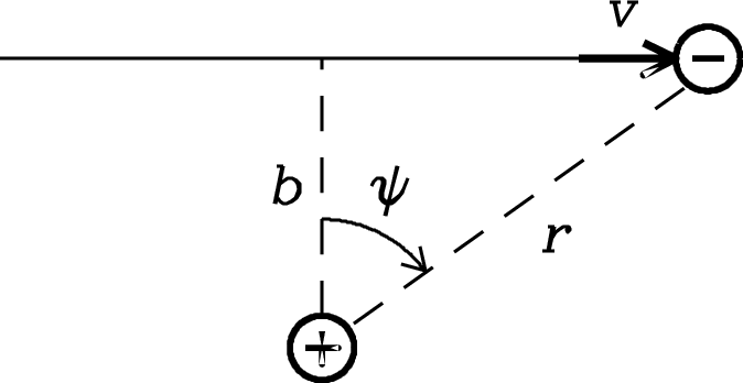
Why should an Hii region emit radio radiation at all? The answer is, because charged particles are being accelerated electrostatically, and nonrelativistic free accelerated charges radiate power according to Larmor’s formula (Equation 2.143). Electrostatic interactions among many kinds of charged particles take place in an Hii region, but most do not emit significant amounts of radiation. The magnitude of the acceleration is inversely proportional to the particle mass . The lightest ion is the hydrogen ion. Its mass is the proton mass g, which is about times the electron mass g. In any electron–ion collision the electron will therefore radiate at least as much power as the ion, so all ionic radiation can be neglected. Interactions between identical particles also do not radiate significantly because the accelerations of the two particles are equal in magnitude but opposite in direction: . Their radiated electric fields are equal in magnitude but opposite in sign, so the net radiated electric field approaches zero at distances much larger than the collision impact parameter (Figure 4.2) and the radiation from electron–electron collisions can be ignored. The bottom line is that only the electron–ion collisions are important, and only the electrons radiate significantly.
4.3.1 Radio Radiation From a Single Electron–Ion Interaction
Figure 4.2 shows an electron passing by a far more massive ion of charge , where for a singly ionized atom such as hydrogen. Each electron–ion interaction will generate a single pulse of radiation. The total energy emitted and the approximate frequency spectrum of the pulse will be derived in this section. The exact spectrum of an individual pulse is not needed because the broad distribution of electron energies and impact parameters smears out spectral details in the total spectrum of an Hii region.
Radio photons are produced by weak interactions because the energy of a radio photon is much smaller than the average kinetic energy of an electron in an Hii region. The numerical comparison below is an example of how astrophysical “intuition” can simplify the electron–ion scattering problem.
The mean electron energy in a plasma of temperature is
| (4.12) |
For an Hii region with K,
| (4.13) |
(This is another useful conversion factor to remember: 1 eV is the typical particle kinetic energy associated with the temperature K.) By comparison, the energy of a radio photon of frequency GHz is only
| (4.14) |
The weak interactions that produce radio photons cause the trajectory of the electron to deflect by only a small angle ( radian). As shown in Figure 4.2, the electron’s path can be approximated by a straight line.
During the interaction, the electron will be accelerated electrostatically both parallel to and perpendicular to its nearly straight path:
| (4.15) | ||||
| (4.16) |
where and is the impact parameter of the interaction, the minimum value of the distance between the electron and the ion.
For any impact parameter , these two equations can be solved to show that the maximum of is a nonnegligible 38% of the maximum of . Even so, the radio radiation arising from is completely negligible. Plotting the variation with time of and during the interaction shows pulses with quite different shapes (Figure 4.3).
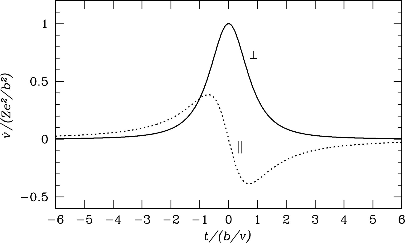
The pulse duration is comparable with the collision time . The pulse is roughly a sine wave of angular frequency , which is much higher than radio frequencies for all relevant impact parameters (Equation 4.43). The parallel acceleration produces some infrared radiation but very little radio radiation. The pulse is a single peak whose frequency spectrum extends from zero up to because the Fourier transform of a Gaussian is also a Gaussian (Appendix B.4), so it is stronger at radio frequencies.
Inserting from Equation 4.16 into Larmor’s formula (Equation 2.143) gives the instantaneous power emitted by the acceleration perpendicular to the electron velocity:
| (4.17) |
The total energy emitted by the pulse is
| (4.18) |
Because for radio photons, the electron velocity is nearly constant. The interaction diagram in Figure 4.2 shows that
| (4.19) |
so
| (4.20) |
and
| (4.21) |
Inserting Equations 4.17 and 4.21 into 4.18 gives
| (4.22) |
The integral in Equation 4.22 is evaluated in Appendix B.7; it is
| (4.23) |
Thus the pulse energy radiated by a single electron–ion interaction characterized by impact parameter and velocity is
| (4.24) |
This energy is emitted in a single pulse of duration , so the pulse power spectrum (Appendix A.4) is nearly flat over all frequencies and falls rapidly at higher frequencies. It is possible to calculate the actual Fourier transform of the pulse shape (solid curve in Figure 4.4), but doing so would only add an unnecessary complication to an already complicated calculation. The ranges of velocities and impact parameters characterizing electron–ion interactions in an Hii region are so wide that averaging over all collision parameters will wash out fine details in the spectrum associated with any particular and .
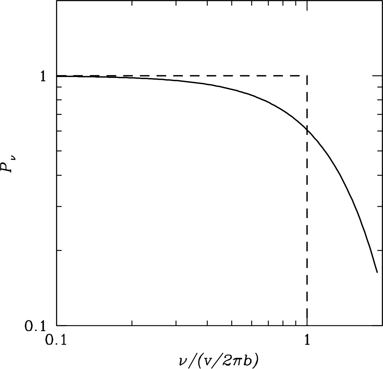
The typical electron speed in a K Hii region is and the minimum impact parameter is cm, so Hz, much higher than radio frequencies. In the approximation that the power spectrum is flat out to and zero at higher frequencies (dashed line in Figure 4.4), the average energy per unit frequency emitted during a single interaction is approximately
| (4.25) |
which simplifies to
| (4.26) |
4.3.2 Radio Radiation From an Hii Region
The strength and spectrum of radio emission from an Hii region depends on the distributions of electron velocities and collision impact parameters (Figure 4.2). The distribution of depends on the electron temperature . The distribution of depends on the electron number density (cm) and the ion number density (cm).
In LTE, the average kinetic energies of electrons and ions are equal. The electrons are much less massive, so their speeds are much higher and the ions can be considered nearly stationary during an interaction (Figure 4.5).
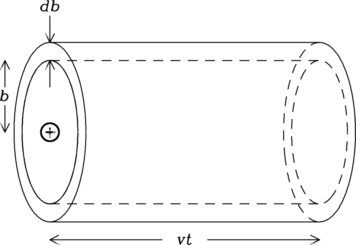
The number of electrons passing any ion per unit time with impact parameter to and speed range to is
| (4.27) |
where is the normalized () speed distribution of the electrons. The number of such collisions per unit time per unit volume per unit velocity per unit impact parameter is
| (4.28) |
The spectral power at frequency emitted isotropically per unit volume is , where is the emission coefficient defined by Equation 2.26. Thus
| (4.29) |
Substituting the results for (Equation 4.26) and (Equation 4.28) into Equation 4.29 gives
| (4.30) | ||||
| (4.31) |
Equation 4.31 exposes a problem: the integral
| (4.32) |
diverges logarithmically. There must be finite physical limits and (to be determined) on the range of the impact parameter that prevent this divergence:
| (4.33) |
The distribution of electron speeds in LTE is the nonrelativistic Maxwellian distribution (see Appendix B.8 for its derivation):
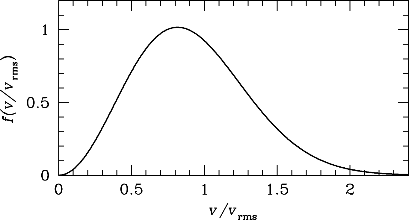
| (4.34) |
Equation 4.34 can be used to evaluate the integral over the electron speeds in Equation 4.33:
| (4.35) |
Substituting so gives
| (4.36) | ||||
| (4.37) | ||||
| (4.38) |
In conclusion, the free–free emission coefficient can be written as
| (4.39) |
The remaining problem is to estimate the minimum and maximum impact parameters and . These estimates don’t have to be very precise because only their logarithms appear in Equation 4.39.
To estimate the minimum impact parameter , notice that the net impulse (change in momentum) during a single electron–ion interaction
| (4.40) |
comes entirely from the perpendicular component of the electric force because the contribution from is antisymmetric about (Figure 4.3). Inserting from Equation 4.16 into Equation 4.40 gives
| (4.41) |
Using Equation 4.21 to change the variable of integration from to gives
| (4.42) |
The maximum possible momentum transfer during the free–free interaction is twice the initial momentum of the electron, so the impact parameter of a free–free interaction cannot be smaller than
| (4.43) |
This result is based on a purely classical treatment of the interaction (see also Jackson [56, section 13.1 and problem 13.1] for a more detailed discussion). The uncertainty principle () implies an independent quantum-mechanical limit
| (4.44) |
but this lower limit is generally smaller than the classical limit in Hii regions and hence may be ignored. This claim can be tested by computing the ratio of the classical to quantum limits for the rms electron velocity :
| (4.45) |
In an Hii region with K and , this ratio , so the classical limit is stronger. Only in much cooler ( K) plasmas is the quantum-mechanical limit important.
There are two effects that might determine the upper limit to the impact parameter. Because electrostatic forces always dominate gravity on small scales, electrons in the vicinity of a nearly stationary ion are free to rearrange themselves to neutralize, or shield, the ionic charge. The characteristic scale length of this shielding is called the Debye length. From Jackson [56], the Debye length is
| (4.46) |
The Debye length is quite large in the low-density plasma of a typical Hii region. For example, if K and ,
| (4.47) |
An independent upper limit to the impact parameter is the largest value of that can generate a significant amount of power at some relevant radio frequency . Recall that the pulse power per unit bandwidth is small above angular frequency so
| (4.48) |
is the maximum impact parameter capable of emitting significant power at frequency .
The controlling upper limit in any particular situation is the smaller of these two upper limits. Numerical values for the lower and upper limits in a typical Hii region observed at GHz are derived in the boxed example, and Equation 4.48 gives the smaller .
Our simple estimate of the ratio
| (4.49) |
is very close to the result of the very detailed derivation in Oster [76]. The ratio is of order , which is much greater than the fractional velocity range in the Maxwellian velocity distribution (Figure 4.6). Also note that
| (4.50) |
varies slowly with changes in either or , so small uncertainties in these limits have very little effect on the calculated emission coefficient of an Hii region.
Because the Hii region is in local thermodynamic equilibrium (LTE) at some temperature , Kirchhoff’s law (Equation 2.30) immediately yields the absorption coefficient (Equation 2.18) in terms of the emission coefficient and the blackbody brightness :
| (4.51) |
in the Rayleigh–Jeans limit. Thus
| (4.52) |
The limit (Equation 4.48) is inversely proportional to frequency so the absorption coefficient is not exactly proportional to . A good numerical approximation is .
The total opacity of an Hii region is the integral of along the line of sight, as illustrated in Figure 4.7:
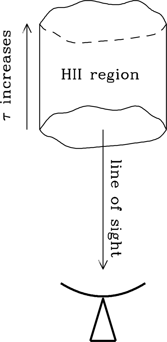
| (4.53) |
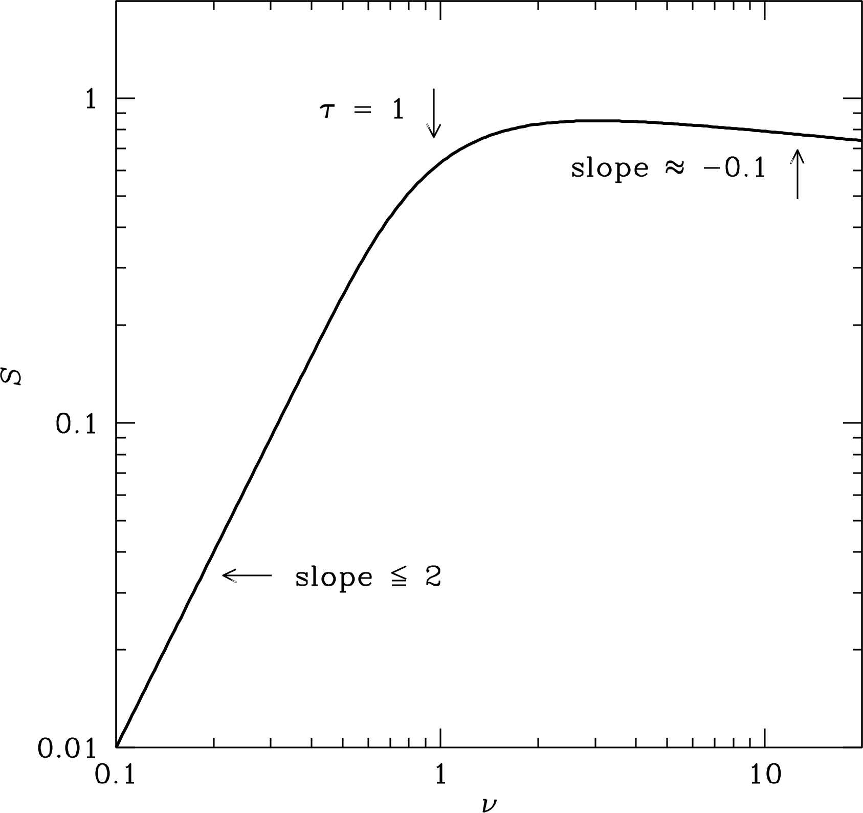
At frequencies low enough that , the Hii region becomes opaque, its spectrum approaches that of a blackbody with brightness temperature approaching the electron temperature ( K), and its flux density obeys the Rayleigh–Jeans approximation . At very high frequencies, , the Hii region is nearly transparent, and
| (4.54) |
On a log-log plot, the overall spectrum of a uniform Hii region looks like Figure 4.8, with the spectral break corresponding to the frequency at which .
The spectral slope on a log-log plot is often called the spectral index and denoted by , whose sign is defined ambiguously:
| (4.55) |
Beware the sign! Unfortunately both sign conventions are found in the literature, and you have to look carefully at each paper to find out which one is being used. With the sign convention, the low-frequency spectral index of a uniform Hii region would be . The sign convention was introduced in the early days of radio astronomy because most sources discovered at low frequencies are stronger at low frequencies than at high frequencies. Thus might mean
| (4.56) |
The () spectral index of any inhomogeneous Hii region will be well above the break frequency, but the break will be more gradual and the low-frequency slope will be somewhat less than just below the break. For example, ionized winds from stars are quite inhomogeneous. Mass conservation in a constant-velocity, isothermal spherical wind implies that the electron density is inversely proportional to the square of the distance from the star: . The low-frequency spectral index of free–free emission by such a wind is closer to than to .
The emission measure (EM) of an Hii region is defined by the integral of along the line of sight expressed in astronomically convenient units:
| (4.57) |
Because is proportional to , the optical depth is proportional to the emission measure. The emission measure is commonly used to parameterize in astronomically convenient units:
| (4.58) |
where the free–free Gaunt factor [18] is a parameter that absorbs the weak frequency dependence associated with the logarithmic term in :
| (4.59) |
Mezger and Henderson [73] found a very good approximation for the free–free opacity that is easy to evaluate numerically:
| (4.60) |
Mezger and Henderson [73, Table 6] lists the errors introduced by this approximation over wide ranges of temperature and frequency.
From the optical depth and the electron temperature it is possible to calculate the brightness temperature
| (4.61) |
of free–free emission. The line-of-sight structure of an Hii region is not normally known, so it is common to approximate the geometry of an Hii region by a circular cylinder whose axis lies along the line of sight, and whose axis length equals its diameter. Suppose further that the temperature and density are constant throughout this volume. Then it is very easy to estimate physical parameters of the Hii region (e.g., electron density, temperature, emission measure, production rate of ionizing photons) from the observed radio spectrum, once the distance to the Hii region is known.
A useful approximation relating the production rate of ionizing photons to the free–free spectral luminosity at the high frequencies where of an Hii region in ionization equilibrium is [95]
| (4.62) |
Free–free emission accounts for about 10% of the 1 GHz continuum luminosity in most spiral galaxies. It is the strongest component in the frequency range from GHz to GHz, above which thermal emission from cool dust grains dominates (Figure 2.24). Free–free absorption flattens the low-frequency spectra of spiral galaxies, and the frequency at which is higher in galaxies with high star-formation rates, especially if the star formation is confined to a compact region near the nucleus. If the free–free and synchrotron emission from a starburst galaxy are roughly cospatial, its radio brightness temperature at frequencies GHz is [30]
| (4.63) |
where K and is the spectral index of the synchrotron radiation. Free–free absorption of the synchrotron radiation limits the maximum brightness temperature to K at frequencies GHz. This limit can be used to identify the energy source powering a compact radio source at the center of a galaxy: if its brightness temperature is significantly higher than K, it is powered by an AGN, not a compact starburst.