Chapter 6 Pulsars
6.1 Pulsar Properties
Pulsars are magnetized neutron stars that appear to emit periodic short pulses of radio radiation with periods between 1.4 ms and 8.5 s. The radical proposal that neutron stars even exist was made with trepidation by Baade & Zwicky in 1934 [5]: “With all reserve we advance the view that a supernova represents the transition of an ordinary star into a new form of star, the neutron star, which would be the endpoint of stellar evolution. Such a star may possess a very small radius and an extremely high density. As neutrons can be packed much more closely than ordinary nuclei and electrons, the ‘gravitational packing’ energy in a cold neutron star may become very large, and, under certain circumstances, may far exceed the ordinary nuclear packing fractions.”
The name pulsar blends “pulse” and “star,” but pulsars are not pulsating stars. Like lighthouses, they continuously emit rotating beams of radiation and appear to flash each time the beam sweeps across the observer’s line of sight. The pulse periods are quite stable because they equal the rotation periods of massive neutron stars. Even though their radio emission mechanism is not well understood, pulsars have become uniquely valuable astrophysical tools:
-
1.
Neutron stars are physics laboratories sampling extreme conditions—deep gravitational potentials , densities exceeding those in atomic nuclei, and magnetic field strengths as high as or even gauss—not reproducible on Earth.
-
2.
Pulse periods can be timed with fractional errors as small as . Accurate pulsar timing permits exquisitely sensitive measurements of quantities such as the power of gravitational radiation emitted by a pulsar in a binary system, neutron-star masses, general relativistic effects in strong gravitational fields, orbital perturbations from binary companions as light as planets, accurate pulsar positions and proper motions, and potentially the distortions of interstellar space produced by long-wavelength gravitational radiation from the mergers of supermassive black holes throughout the universe.
Lorimer and Kramer [70] and Lyne and Graham-Smith [71] have written excellent reference books about pulsars and their astrophysical applications.
6.1.1 Discovery
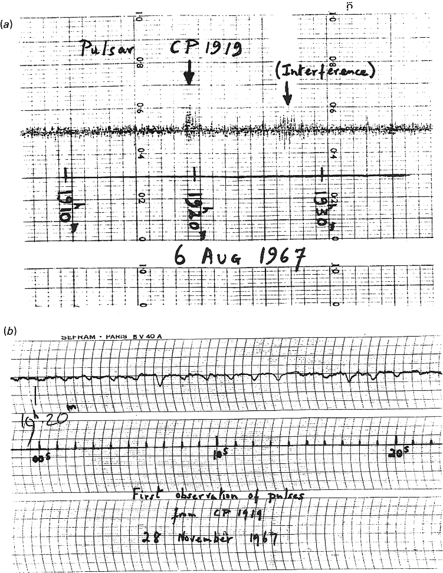
Pulsars were discovered [50] serendipitously in 1967 on chart recordings (Figure 6.1) obtained during a low-frequency ( MHz) search for compact extragalactic radio sources that scintillate in the interplanetary plasma, just as stars twinkle in the Earth’s atmosphere.
This history of this important discovery is a warning against overprocessing data before looking at them, ignoring unexpected signals, and failing to explore the observational “parameter space” covered by the data—here the relevant parameter being time. The strong pulsar PSR B0329+54 was clearly visible in 1954 survey data from the Jodrell Bank 250-foot radio telescope [71], but nobody paid any attention to it at the time. The X-ray pulsar in the Crab Nebula (Figure 8.10) was present in data taken several months before the discovery of radio pulsars, but only after the radio pulsar in the Crab Nebula was announced were the X-ray pulses extracted [39]. As radio instrumentation and data-processing software become more sophisticated, more data are “cleaned up” automatically before they reach the astronomer. Matched filtering that brings out the expected signal usually suppresses the unexpected. Thus, clipping circuits or software remove the strong impulses that are usually caused by terrestrial interference, and integrators smooth out fluctuations shorter than the integration time. Most pulses seen by radio astronomers are just artificial interference from radar, electric cattle fences, etc., and short pulses from sources at interstellar distances imply unexpectedly high brightness temperatures , which is much higher than the K upper limit for incoherent electron-synchrotron radiation imposed by synchrotron self-Compton cooling (Section 5.5.3).
Cambridge University graduate student Jocelyn Bell recognized that pulsars are astronomical sources where others had failed because she noticed that some “scruffy” pulses in her chart-recorder data (Figure 6.1) didn’t look like other forms of interference and they reappeared exactly once per sidereal day, indicating an origin outside the Solar System. Fortunately, she and her supervisor, Antony Hewish, “decided initially not to computerize the output because until we were familiar with the behavior of our telescope and receivers we thought it better to inspect the data visually, and because a human can recognize signals of different character whereas it is difficult to program a computer to do so.” Read http://www.bigear.org/vol1no1/burnell.htm for the full discovery story in her own words.
6.1.2 Neutron Star Masses and Densities
The sources of the pulses were originally unknown, and even intelligent transmissions by “LGM” (Little Green Men) were seriously suggested as explanations for pulsars. Their short periods imply very compact sources such as white dwarf stars, black holes, and neutron stars; their stable periods rule out black holes. Astronomers were familiar with slowly varying or pulsating emission from stars, but the natural period of a radially pulsating star depends on its mean density and is typically days, not seconds. There is a comparable lower limit to the rotation period of a gravitationally bound star, set by the requirement that the centrifugal acceleration at its equator not exceed the gravitational acceleration. If a nearly spherical star of mass and radius rotates with angular velocity ,
| (6.1) |
implies
| (6.2) |
In terms of the mean density
| (6.3) | |||
| (6.4) |
and
| (6.5) |
Equation 6.5 gives a conservative lower limit to the mean density because a rapidly spinning star is oblate, which increases the centrifugal acceleration and decreases the gravitational acceleration at its equator.
The first pulsar discovered has a period s, so its mean density is at least
This limit is just consistent with the known densities of white dwarf stars. But soon the faster ( s) pulsar in the Crab Nebula was discovered, and its period implies a density much higher than any stable white-dwarf star supported by electron-degeneracy pressure. Also, the Crab Nebula (Figure 8.10) is the remnant of a supernova recorded by Chinese astronomers as a “guest star” in 1054 AD, so the discovery of this pulsar confirmed the suggestion by Baade and Zwicky [5] that neutron stars are the compact remnants of supernovae. The fastest known pulsar has s implying g cm, the density of atomic nuclei.
A star whose mass is greater than the Chandrasekhar mass
| (6.6) |
cannot be supported by electron degeneracy pressure and will collapse to become a neutron star. Equation 6.2 implies the maximum radius
| (6.7) |
of a s pulsar with mass is
| (6.8) |
These numbers motivate the definition of the canonical neutron star as being a uniform density sphere with mass , radius km, and moment of inertia . “Canonical” is perhaps too strong a term for what is really no more than a convention for the typical properties of neutron stars; individual neutron stars can have different masses and radii. The extreme density and pressure turn most of the star into a neutron superfluid that is a superconductor at temperatures up to K. The masses of individual pulsars have been measured with varying degrees of accuracy, and many are close to the canonical . The highest accurately measured pulsar masses are , and they rule out all currently proposed hyperon or boson condensate equations of state and “free” quarks [34]. Any neutron star of significantly higher mass ( in standard models) must collapse and become a black hole.
6.1.3 Magnetic Fields
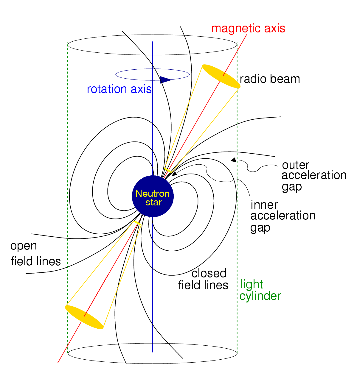
The Sun and many other stars are known to possess approximately dipolar magnetic fields. Stellar interiors are fully ionized and hence good electrical conductors. Charged particles are constrained to move along magnetic field lines, and magnetic field lines are tied to the charged particles. When a star collapses from a radius km to km, its cross-sectional area is divided by , its magnetic flux (where is the unit vector normal to each infinitesimal surface area ) is conserved, and the magnetic field strength is multiplied by . An initial magnetic field strength G becomes G after collapse, so young neutron stars should have very strong dipolar fields. The best models of the core-collapse process show that a dynamo effect can generate even stronger magnetic fields. Such dynamos may be able to produce the – G fields observed in magnetars, which are neutron stars having such strong magnetic fields that their radiation is powered by magnetic field decay. Conservation of angular momentum during collapse increases the rotation rate by about the same factor, , yielding initial rotation periods in the millisecond range. Thus young neutron stars should contain rapidly rotating magnetic dipoles (Figure 6.2).
6.1.4 Magnetic Dipole Radiation
If a rotating magnetic dipole is inclined by some inclination angle from the rotation axis, it emits electromagnetic radiation at the rotation frequency. Rewriting the Larmor formula (Equation 2.143) in terms of power radiated by a rotating electric dipole gives
| (6.9) |
where is the electric dipole moment and is its component perpendicular to the rotation axis. J. J. Thomson’s derivation of the Larmor formula in terms of electric field lines (Section 2.7) is also valid for magnetic field lines. The Gaussian CGS units for magnetic and electric field are the same, so the power of magnetic dipole radiation is
| (6.10) |
where is the perpendicular component of the magnetic dipole moment. For a uniformly magnetized sphere with radius and surface magnetic field strength , the magnitude of the magnetic dipole moment is [56]
| (6.11) |
If the inclined magnetic dipole rotates with angular velocity , then
| (6.12) |
where is the pulsar period. This electromagnetic radiation will appear at the very low radio frequency kHz, so low that it cannot propagate through the surrounding ionized nebula or ISM. Magnetic dipole radiation extracts rotational kinetic energy from the neutron star and causes the pulsar period to increase with time. The absorbed radiation deposits energy in the surrounding nebula, the Crab Nebula (Figure 8.10) being a prime example.
6.1.5 Spin-Down Luminosity
The rotational kinetic energy of a spinning object is related to its moment of inertia by
| (6.13) |
The moment of inertia of a small mass element about any rotation axis is its mass multiplied by the square of its radial distance from the rotation axis. The moment of inertia of a sphere with radius , mass , and uniform density spinning about its -axis is obtained by summing over its mass elements:
| (6.14) |
where is the distance from the rotation axis and is the height in cylindrical coordinates centered on the sphere. Then
| (6.15) |
The moment of inertia of a canonical neutron star is
| (6.16) |
The rotational kinetic energy of a canonical neutron star with the rotation period s of the Crab pulsar is
As magnetic dipole radiation extracts rotational energy, it slowly increases the period of a pulsar:
| (6.17) |
Note that the period derivative is a dimensionless (seconds per second) pure number. Combining the observed period and period derivative yields an estimate of the rate at which the rotational energy is changing. The quantity
| (6.18) |
is called the spin-down luminosity. It is not a measured luminosity; it is the measured loss rate of rotational energy, which is presumed to equal the luminosity of magnetic dipole radiation. The spin-down luminosity is usually expressed in terms of the pulse period :
| (6.19) |
and Equation 6.18 becomes
| (6.20) |
The Crab pulsar has s and . If (Equation 6.16), its spin-down luminosity is
If , the luminosity of the low-frequency () magnetic dipole radiation from the Crab pulsar is comparable with the entire radio output of our Galaxy! It even exceeds the Eddington luminosity limit (Section 5.4.2) of the neutron star, which is possible because the energy source is not accretion. It greatly exceeds the average radio pulse luminosity of the Crab pulsar, . The long wavelength ( m) magnetic-dipole radiation is absorbed by and heats up the surrounding Crab Nebula (Figure 8.10), making it the “megawave oven” counterpart of a kitchen microwave oven. The observed bolometric luminosity of the Crab Nebula is comparable with the spin-down luminosity, supporting the model that rotational kinetic energy is converted to magnetic dipole radiation that is absorbed by the surrounding ionized nebula and later reradiated at radio through X-ray wavelengths.
6.1.6 Minimum Magnetic Field Strength
If , Equations 6.12 and 6.20 can be combined to yield a lower limit to the magnetic field strength at the neutron star surface, where is the unknown inclination angle between the rotation and magnetic axes:
| (6.21) | |||
| (6.22) | |||
| (6.23) | |||
| (6.24) |
Inserting the constants for the canonical pulsar in CGS units yields for the first factor
| (6.25) |
so the minimum magnetic field strength at the surface of a canonical pulsar is
| (6.26) |
It is sometimes called the characteristic magnetic field of a pulsar.
The minimum magnetic field strength of the Crab pulsar ( s, ) is
This is an amazingly strong magnetic field. Its energy density is
| (6.27) |
Just of this magnetic field contains over of energy, the annual output of a large nuclear power station.
6.1.7 Characteristic Age
If the spin-down luminosity equals the magnetic dipole radiation luminosity and doesn’t change significantly with time, a pulsar’s age can be estimated from on the further assumption that the pulsar’s initial period was much shorter than its current period. Solving Equation 6.23 for shows that
| (6.28) |
also doesn’t change with time. Rewriting the identity as and integrating over the pulsar’s age gives
| (6.29) |
because is constant. Integrating Equation 6.29 gives
| (6.30) |
In the limit , the characteristic age of a pulsar defined by
| (6.31) |
should be close to the actual age of the pulsar. The characteristic age depends only on the observables and ; it does not depend on the unknown radius , moment of inertia , or perpendicular magnetic field . However, a newly formed neutron star with small may be quite oblate and will initially be slowed down by emitting quadrupole gravitational radiation. This can cause the characteristic age to be somewhat larger than the true age for young pulsars.
For example, the characteristic age of the Crab pulsar ( s, ) is
It is slightly larger than the actual age of the Crab pulsar, which is known to be just under because the Crab supernova was observed in 1054 AD.
6.1.8 Braking Index
If magnetic dipole radiation is solely responsible for pulsar spin down, then and Equations 6.12 and 6.18 together imply
| (6.32) |
The pulsar braking index is defined by
| (6.33) |
where is the constant of proportionality. The braking index is completely determined by the observables , , and , so comparing its observed value with the expected provides a useful check on pulsar spin-down models. The time derivative of Equation 6.33 is
| (6.34) |
so
| (6.35) |
Converting from angular velocities to periods with
| yields | |||
| (6.36) | |||
| (6.37) |
the braking index in terms of the observables , , and .
Braking indices in the range have been observed and used to investigate alternative spin-down mechanisms and to make more sophisticated estimates of pulsar ages and initial spin periods [60].
6.1.9 The Lives of Pulsars
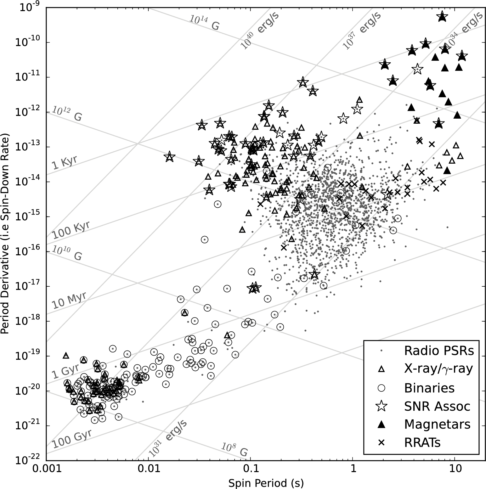
Pulsars are born in supernovae and appear in the upper left corner of the pulsar diagram (Figure 6.3). If is conserved and they age as described above, they gradually move to the right and down, along lines of constant and crossing lines of constant characteristic age. Pulsars with characteristic ages yr are often found in or near recognizable supernova remnants (SNRs). Older pulsars are not, either because their SNRs have faded to invisibility or because the supernova explosions expelled the pulsars with enough speed that they have since escaped from their parent SNRs. The bulk of the pulsar population is older than yr but much younger than the Galaxy ( yr). The observed distribution of pulsars in the diagram indicates that something changes as pulsars age. One controversial possibility is that the magnetic fields of old pulsars must decay on timescales yr, causing old pulsars to move almost straight down in the diagram until either their magnetic field is too weak or their spin rate is too slow to produce radio emission via the normal, and as yet still highly uncertain, emission mechanism. Rotating Radio Transients (RRATs) are pulsars that emit so sporadically that they are more easily detected in searches for single pulses rather than for periodic pulse trains. RRATs with measurable periods usually have (Figure 6.3). Some RRATs may be old pulsars on the verge of becoming radio quiet.
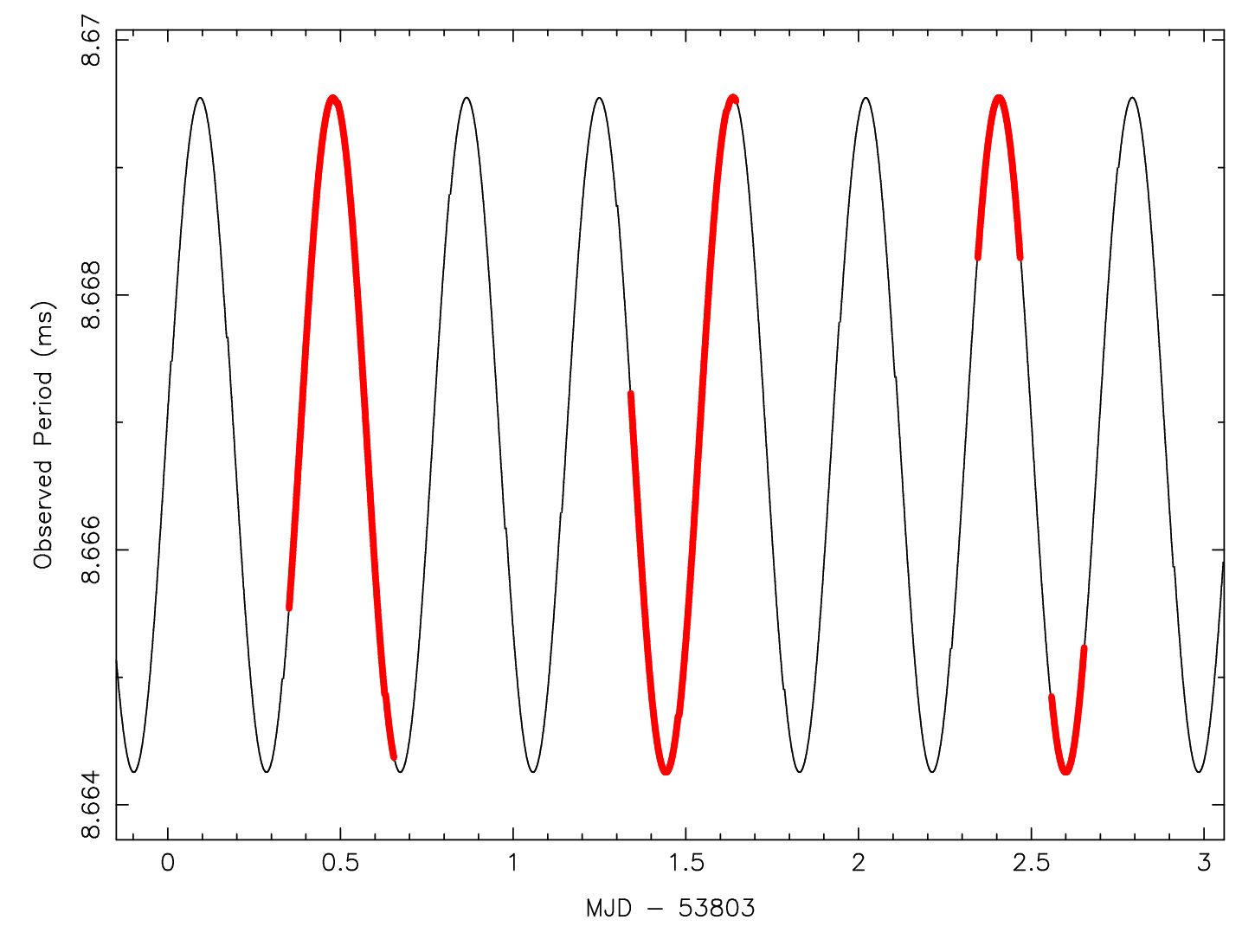
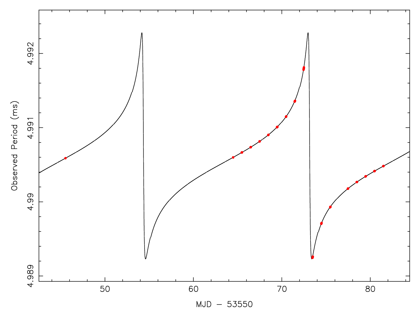
Almost all short period ( s) pulsars having fairly weak magnetic field strengths ( G) are in binary systems, as evidenced by periodic orbital variations in their observed pulse periods (Figure 6.4). These recycled pulsars have been spun up by accreting mass and angular momentum from their stellar companions, to the point that they emit radio pulses despite their relatively low magnetic field strengths G. (Apparently, currents in the accreting plasma “bury” the magnetic field of the neutron star itself.) The magnetic fields of neutron stars funnel the ionized accreting material onto the magnetic polar caps, which become so hot that they, as well as the hot accretion disk, emit X-rays. We observe these systems as the Low Mass X-ray Binaries (LMXBs). As the neutron stars rotate, their inclined magnetic polar caps can appear and disappear from view, causing periodic fluctuations in X-ray flux, and making some of these systems detectable as X-ray pulsars.
 |
 |
Millisecond pulsars (MSPs) with low mass (–) white-dwarf companions typically have orbits with small eccentricities owing to strong tidal dissipation during the accretion phase which spins up the pulsars. The eccentricity of an elliptical orbit is defined as the ratio of the separation of the foci to the length of the major axis. It ranges between for a circular orbit and for a parabolic orbit. Pulsars with extremely eccentric orbits usually have neutron-star companions, indicating that these companions exploded as asymmetric supernovae and nearly disrupted the binary system. Stellar interactions in globular clusters cause a much higher fraction of recycled pulsars per unit mass than in the Galactic disk. These interactions can result in very strange systems such as pulsar–main-sequence-star binaries and MSPs in highly eccentric orbits. In both cases, the original low-mass companion star that recycled the pulsar was ejected in an interaction and replaced by another star.
About 15% of millisecond pulsars are isolated. They were probably recycled via the standard scenario in binary systems, but the energetic MSPs eventually ablated their companions away. Recently, many new “black widow” and “redback” systems have been detected which seem to be doing exactly this. They exhibit eclipses of their radio MSP emission, likely owing to free–free absorption by the ionized gas in the systems being blown off the companion stars.
6.1.10 Emission Mechanisms
The radio pulses originate in the pulsar magnetosphere. Because the neutron star is a spinning magnetic dipole, it acts as a unipolar generator. The total Lorentz force acting on a charged particle is
| (6.38) |
Charges in the magnetic equatorial region redistribute themselves by moving along closed magnetic field lines until they build up an electrostatic field large enough to cancel the magnetic force and give . The induced voltage is about in MKS units. However, the corotating field lines emerging from the polar caps cross the light cylinder (Figure 6.2), an imaginary cylinder centered on the pulsar and aligned with the rotation axis at whose radius the corotating speed equals the speed of light, so these field lines cannot close. Electrons in the polar cap are magnetically accelerated to very high energies along the open but curved field lines, where the acceleration resulting from the curvature causes them to emit curvature radiation that is strongly polarized in the plane of curvature. As the radio beam sweeps across the line of sight, the plane of polarization is observed to rotate by up to 180 degrees, a purely geometrical effect. Normal “slow” pulsars usually have quite large amounts of typically linear polarization. There are several relativistic effects in the rapidly rotating magnetospheres of millisecond pulsars that complicate this emission-geometry-based polarization, yet millisecond pulsars are typically highly polarized as well. High-energy photons produced by curvature radiation interact with the magnetic field and lower-energy photons to produce electron–positron pairs that radiate additional high-energy photons. The final results of this cascade process are bunches of charged particles that emit at radio wavelengths. Pulsars “die” in the lower right corner of the diagram (Figure 6.3) when they have sufficiently low and high that the curvature radiation near the polar surface is no longer capable of generating particle cascades.
The extremely high brightness temperatures of pulsars are explained by coherent radiation. The electrons do not radiate as independent charges ; instead bunches of electrons in volumes whose dimensions are less than a wavelength emit in phase as charges . Larmor’s formula indicates that the power radiated by a charge is proportional to , so the radiation intensity can be times brighter than incoherent radiation from the same total number of electrons. Because the coherent volume is smaller at shorter wavelengths, most pulsars have extremely steep radio spectra. Typical pulsar spectral indices (defined using the positive convention, see Equation 4.55) are (i.e., ), although some can be much steeper (), and a handful are almost flat ().
6.2 Pulsars and the Interstellar Medium
With their sharp and short-duration pulse profiles allowing continuous “on–off” differential measurements, small sizes, and high brightness temperatures, pulsars are unique probes of the interstellar medium (ISM). This section closely follows the discussion in Lorimer and Kramer [70], and Equations 6.39 through 6.42 are derived in Appendix D.
The electrons in the ISM make up a cold plasma whose refractive index is
| (6.39) |
where is the frequency of the radio waves, is the plasma frequency
| (6.40) |
and is the electron number density. For a typical ISM value , kHz. If then is imaginary and radio waves cannot propagate through the plasma.
For propagating radio waves, and the group velocity
| (6.41) |
of pulses is less than the vacuum speed of light. For most radio observations , so
| (6.42) |
A broadband pulse moves through a plasma more slowly at lower frequencies than at higher frequencies. If the distance to the source is , the dispersion delay at frequency is
| (6.43) | ||||
| (6.44) |
In astronomically convenient units the dispersion delay is
| (6.45) | |||
| where | |||
| (6.46) | |||
in units of pc cm is called the dispersion measure and represents the integrated column density of electrons between the observer and the pulsar.
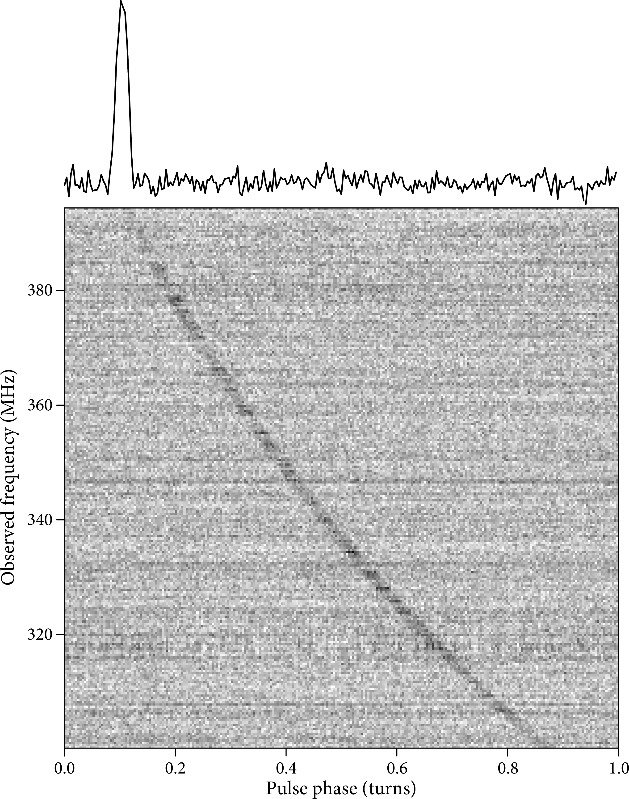
Because pulsar observations almost always cover a wide bandwidth, uncorrected differential delays across the band cause dispersive smearing of the pulsed signal when integrated across the band. If uncorrected, the delays would smear out the integrated pulse in time and make most pulsars undetectable (see Figure 6.5). For pulsar searches, the DM is unknown a priori and is a search parameter much like the pulsar spin frequency. This extra search dimension is one of the primary reasons that pulsar searches are computationally intensive. For high-precision timing observations of pulsars with known DMs, if Nyquist-sampled voltage data (often called “baseband” data) are available, the dispersion may be completely removed from the data by a technique known as coherent dedispersion. The dispersed data are de-convolved using the complex conjugate of the complex transfer function of the ISM that caused the dispersion in the first place.
Dispersion measures can be used to provide distance estimates to pulsars. Crude distances can be calculated for pulsars near the Galactic plane by assuming that . However, several sophisticated models of the Galactic electron-density distribution now exist (e.g., NE2001; Cordes and Lazio [33]) that provide much better ( or less) distance estimates.
The ionized ISM affects pulsar signals in several other ways besides dispersion. Inhomogeneities in the turbulent ISM result in both diffractive and refractive scintillation, or time- and frequency-dependent flux-density variations of the pulsar signal much like the “twinkling” of starlight by Earth’s turbulent atmosphere. Diffractive scintillations occur over typical timescales of minutes to hours and radio bandwidths of kHz to hundreds of MHz, and they can cause more than order-of-magnitude flux-density fluctuations. Refractive scintillations tend to be less than a factor of 2 in amplitude and occur on timescales of weeks.
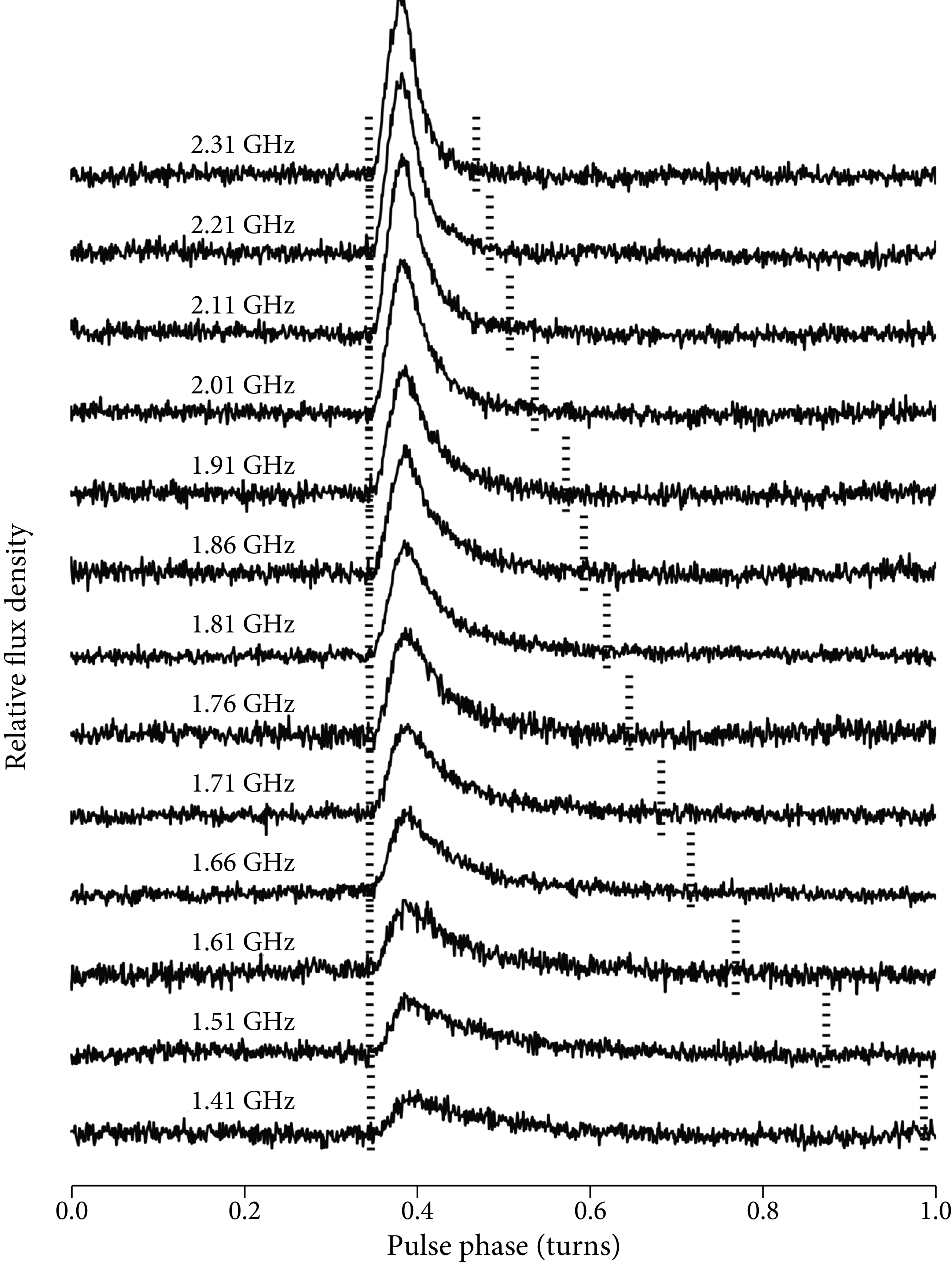
A phenomenon related to scintillation is pulse broadening caused by scattering of radio waves. ISM inhomogeneities cause multipath propagation of a pulsar signal, whereby some rays travel longer physical distances because they do not follow straight lines to the observer. Such rays are delayed in time relative to those traveling more direct paths, and so cause a strongly frequency-dependent (typically ) exponential-like scattering tail of the pulse (see Figure 6.6). This scatter broadening can greatly decrease both the observed pulsed flux density from a pulsar and its timing precision.
Finally, pulsars have broadband continuum spectra, so if there are gas clouds along our line of sight, pulsars can be used to probe the ISM via absorption by spectral lines of Hi or molecules. Such absorption spectra can be used to estimate pulsar distances.
6.3 Pulsar Timing
Pulsars are intrinsically interesting and exotic objects, but much of the best science based on pulsar observations has come from their use as tools via pulsar timing. Pulsar timing is the regular monitoring of the rotation of the neutron star by tracking (nearly exactly) the arrival times of the radio pulses. The key point to remember is that pulsar timing unambiguously accounts for every single rotation of the neutron star over long periods (years to decades) of time. This unambiguous and very precise tracking of rotation phase allows pulsar astronomers to probe the interior physics of neutron stars, make extremely accurate astrometric measurements, uniquely test gravitational theories in the strong-field regime, and possibly within the next few years, directly detect gravitational waves (GWs) (GWs are propagating distortions of space–time) from supermassive black hole binaries.
For pulsar timing, astronomers “fold” (average) the data from many pulses modulo the instantaneous pulse period . The instantaneous pulse frequency is , and the instantaneous pulse phase is defined by . Pulse phase is usually measured in turns of radians, so .
Averaging over many pulses yields an average pulse profile. Although the shapes of individual pulses vary considerably because pulsar emission is intrinsically a noise process, the shape of the average profile is quite stable.
For timing, the average pulse profile is correlated with a template or model profile so that its phase offset can be determined. When multiplied by the instantaneous pulse period, that phase yields a time offset that can be added to a high-precision reference point on the profile (for example, the left edge of the profile based on the recorded time of the first sample of the observation) to create the time of arrival (TOA).
The precision with which a TOA can be determined is approximately equal to the duration of a sharp pulse feature (e.g., the leading edge) divided by the signal-to-noise ratio of the average profile. It is usually expressed in terms of the width of the pulse features in units of the pulse period , and the signal-to-noise ratio such that . Strong, fast pulsars with narrow pulse profiles provide the most accurate arrival times.
In the nearly inertial frame of the Solar System barycenter (center of mass), the rotation period of a pulsar is nearly constant, so the time-dependent phase of a pulsar can be approximated by the Taylor expansion
| (6.47) |
where and are arbitrary reference phases and times for each pulsar. The critical constraint for pulsar timing is that the observed rotational phase difference between each of the TOAs must contain an integer number of rotations. Each TOA corresponds to a different time , so the correct fitting parameters (e.g., and ) must result in a phase change between each pair of TOAs and that is an integer number of turns, or turns. Because all measurements are made with regard to the integrated pulse phase rather than the instantaneous pulse period, the precision with which astronomers can make long-term timing measurements can be quite extraordinary.
With what precision can timing determine the spin frequency of a pulsar? Because when is measured in turns, the precision is based on how precisely a change in phase can be measured over some time interval . Typically, is the length of time (up to several tens of years for many pulsars now) over which a pulsar’s phase has been tracked through regular monitoring. is determined principally by the individual TOA precisions, although for some types of measurements a statistical component is important as well because precision improves as the number of measurements if the random errors are larger than the systematic errors. For example, the original millisecond pulsar B193721 has pulse period s and the TOA precision is s, which corresponds to a phase error of turns. This pulsar has been timed for years, so
| (6.48) |
That pulsar’s spin frequency is 642 Hz, so the absolute frequency error implies that the spin rate is known to 15 significant figures!
Many corrections have to be applied to the observed TOAs before can be expressed as a Taylor series (Equation 6.47). The arrival of a pulse at an observatory on Earth at topocentric (topocentric means measured from a fixed point on the Earth’s surface) time can be corrected to the time in the nearly inertial Solar System barycentric frame, which we assume to be nearly the same as the time in the frame comoving with the pulsar. Note that the measured pulse rates will differ from the actual pulse rates in the pulsar frame by the Doppler factor resulting from the unknown line-of-sight pulsar velocity as well as unknown relativistic corrections from within the pulsar system itself.
The principal terms in the timing equation are
| (6.49) |
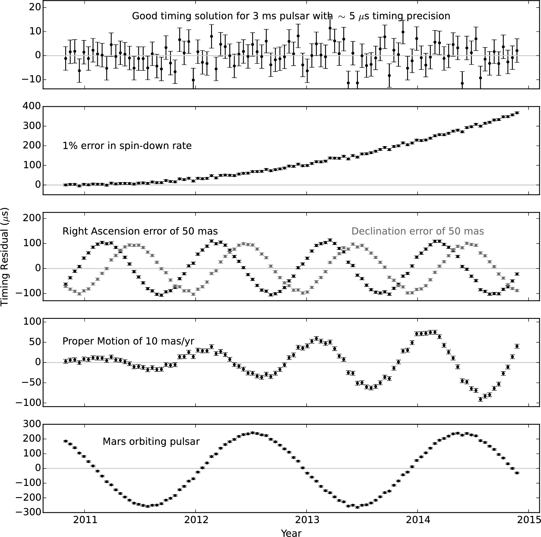
As before, is a reference epoch, represents a clock correction that accounts for differences between the observatory clocks and terrestrial time standards, and is the frequency-dependent dispersion delay caused by the ISM. The other terms are delays from within the Solar System and, if the pulsar is in a binary, from within its orbit. The Roemer delay is the classical light travel time across the Earth’s orbit. Its magnitude is s, where is the ecliptic latitude of the pulsar (the angle between the pulsar and the ecliptic plane containing the Earth’s orbit around the Sun), and is the corresponding delay across the orbit of a pulsar in a binary or multiple system. The Einstein delay accounts for the time dilation from the moving pulsar (and observatory) and the gravitational redshift caused by the Sun and planets or the pulsar and any companion stars. The Shapiro delay is the extra time required by the pulses to travel through the curved space–time containing the Sun, planets, and pulsar companions. Errors in any of these parameters, as well as other parameters such as , , and proper motion, give very specific systematic signatures in plots of timing residuals (see Figure 6.7), which are simply the differences between the observed TOAs and the predicted TOAs based on the current timing model parameters.
A good example showing how pulsar timing can be extremely useful is timing-based pulsar astrometry. Pulsar positions on the sky are determined by timing a pulsar over the course of a year as the Earth orbits the Sun and tracking the changing Roemer delay.
The Roemer delay of a pulsar at ecliptic coordinates (ecliptic longitude) and (ecliptic latitude) is
| (6.50) |
where is the orbital phase of the Earth with respect to the vernal equinox (the intersection of the ecliptic plane and the celestial equator). Equation 6.50 is only approximate because the Earth’s orbit is not quite circular.
If there is an error in our position estimate, the individual position error components and cause a differential time delay to be present in the timing residuals with respect to the correct Roemer delay:
| (6.51) |
If the position errors are small enough that , , and , we can use trigonometric angle-sum identities and then simplify to get
| (6.52) |
Applying the trig identity to the equation for , we see that
| (6.53) | |||
| (6.54) |
and therefore
| (6.55) | |||
| (6.56) |
where and are the amplitude (in time units because it corresponds to light-travel time delay) and phase of an error sinusoid that we would observe in the timing residuals from the pulsar (see the middle panel in Figure 6.7).
If the pulsar is located near the ecliptic plane (), then and there is maximum timing leverage, and therefore minimum error, in the determination of . However, and so the errors on are huge. A similar problem occurs near the ecliptic pole for . VLBI positions give better astrometric accuracy for pulsars near the ecliptic plane or ecliptic pole.
In a timing fit for position, the amplitude of the error sinusoid in the timing residuals as described above will be determined to an absolute precision approximately equal to the TOA uncertainty divided by the square-root of the number of observations made of the pulsar (so long as there is at least one year of timing data).
For binary pulsars, the time delays across the neutron-star orbit allow for similar high-precision measurements of the pulsar orbital parameters. The binary pulsar Roemer delays comprise up to five Keplerian parameters describing elliptical orbits: the projected semimajor axis , the longitude of periastron , the time of periastron passage , the orbital period , and the orbital eccentricity .
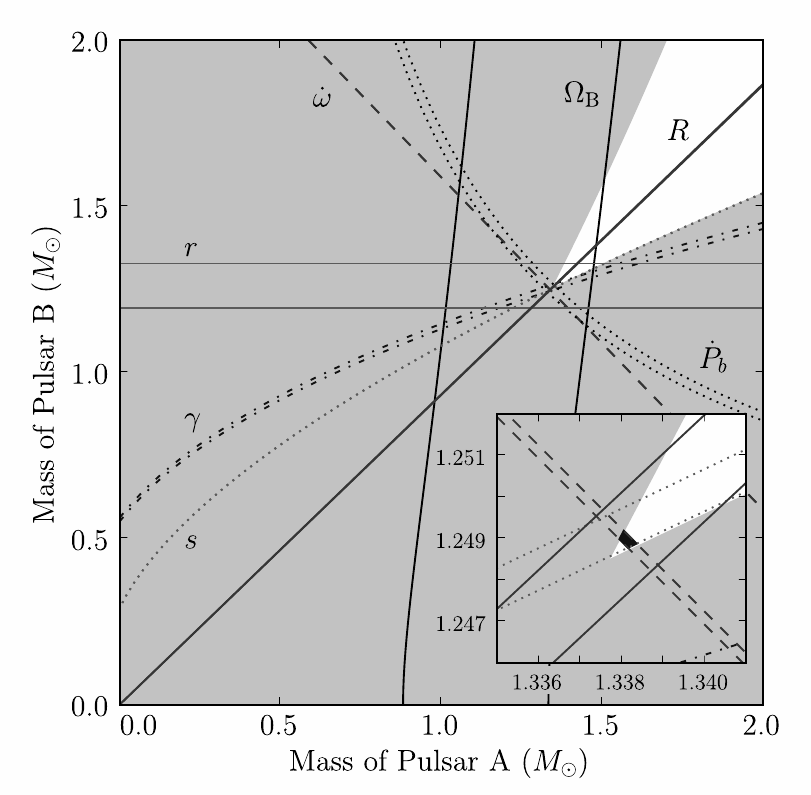
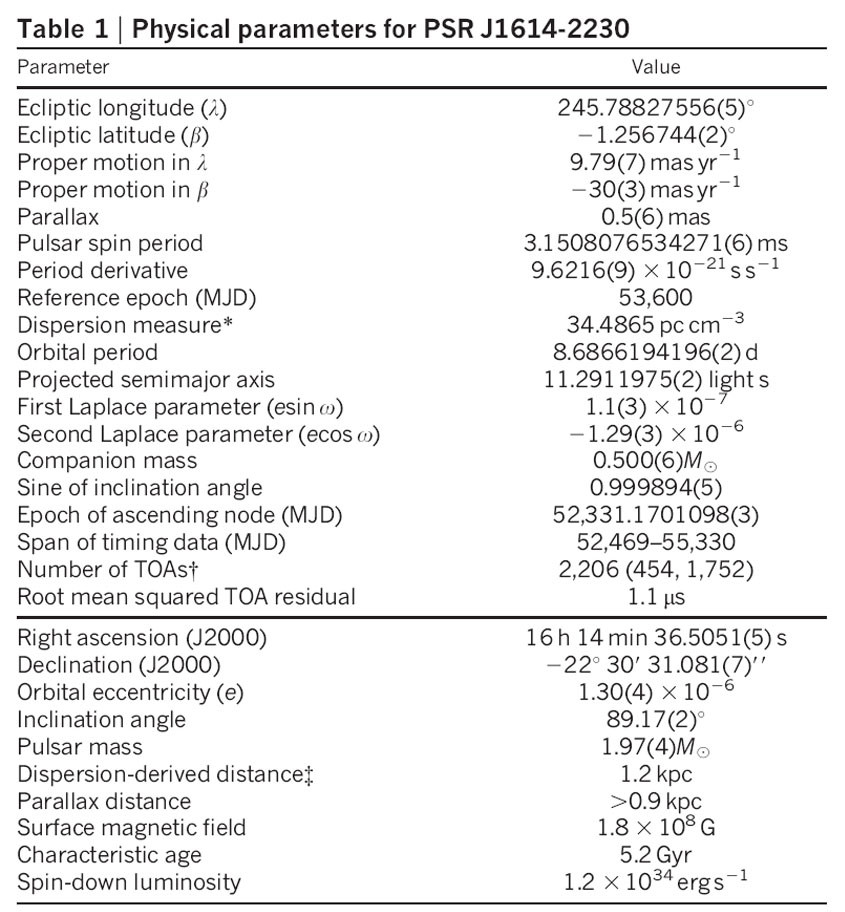
Relativistic binaries, particularly those with compact and elliptical orbits, may allow the measurement of up to five post-Keplerian (PK) parameters: the rate of periastron advance (elliptical orbits do not close in relativistic theories), the orbital period decay caused by the emission of gravitational radiation, the relativistic term describing time dilation and gravitational redshift, and the Shapiro delay terms (range) and (shape). An example of a full “timing solution,” listing high-precision spin, astrometric, binary, and two post-Keplerian parameters , is shown in Figure 6.8.
In any theory of gravity, the five PK parameters are functions only of the pulsar mass , the companion mass , and the standard five Keplerian orbital parameters. For general relativity, the formulas are
| (6.57) | ||||
| (6.58) | ||||
| (6.59) | ||||
| (6.60) | ||||
| (6.61) |
In these equations, s is the solar mass in time units (which is known much more precisely than either or individually), , , and are in solar masses, and (where is the orbital inclination). If any two of these PK parameters are measured, the masses of the pulsar and its companion can be determined. If more than two are measured, each additional PK parameter yields a different test of a gravitational theory.
For the famous case of the Hulse–Taylor binary pulsar B191316, high-precision measurements of and were first made to determine the masses of the two neutron stars accurately. The Nobel-prize-winning measurement came with the eventual detection of , which implied that the orbit was decaying in accordance with general relativity’s predictions for the the emission of gravitational radiation.
More recently, the double-pulsar system J07373039 was discovered, which contains two pulsar clocks in a more compact orbit (2.4 hrs compared to 7.7 hrs for PSR B1913+16), allowing the measurement of all five PK parameters as well as the pulsar mass ratio and relativistic spin precession, giving a total of five tests of general relativity. Kramer et al. [62] showed that general relativity is correct at the 0.05% level and measured the masses of the two neutron stars to within 1 part in , and the measurements continue to improve (see Figure 6.9).
The double neutron-star systems have indirectly confirmed the existence of gravitational waves by matching the predicted orbital decays as orbital energy is carried away by gravitational radiation. But over the last decade, one of the driving efforts in pulsar astronomy has become the direct detection of GWs using pulsar timing arrays (PTAs). A PTA is an array of MSPs spread over the sky rather than an array of telescopes, and the goal is to use that pulsar array to detect correlated signals in the timing residuals of dozens of MSPs caused by the distortions of interstellar space from nanohertz (i.e., periods of years) GWs passing through our Galaxy.
Because GW emission and propagation is a quadrupolar process in general relativity, in contrast to the dipolar emission of electromagnetic waves from an accelerating electron, GWs cause specific angular correlations in the timing residuals between pairs of pulsars on the sky. Pulsars close together on the sky will be similarly affected by a passing GW, whereas those much farther apart on the sky will be uncorrelated or even negatively correlated by the same GW. That angular pattern is known as the Hellings and Downs curve [49], and detecting it would be the key to confirming that correlated signals in timing residuals are caused by GWs and not by other effects such as clock or planetary ephemeris errors.
The most likely sources of detectable nanohertz GWs are supermassive black hole binaries (with total masses of – M) and years-long orbital periods after their parent galaxies have merged. A single massive nearby system, or an ensemble of more distant, less massive systems (making a “stochastic background” of GWs), will cause tens-of-nanosecond spatially and temporally correlated systematics in PTA timing residuals. This level of long-term timing precision for the best MSPs is now being achieved.
Three PTA experiments have been working on this endeavor: NANOGrav in North America and the Parkes and European PTAs in Australia and Europe, respectively. Together, they are collaborating in the International Pulsar Timing Array (IPTA), and huge progress toward a detection has been made recently. Current PTA limits, based on upper limits for appropriately correlated low-frequency timing residuals, are beginning to constrain models of galaxy mergers throughout the universe. And given continued improvements in pulsar timing capability and many new high-precision MSPs from recent surveys, a direct detection of GWs seems possible or even likely within the next five years.