Chapter 1 Introduction
1.1 An Introduction to Radio Astronomy
1.1.1 What Is Radio Astronomy?
Radio astronomy is the study of natural radio emission from celestial sources. The range of radio frequencies or wavelengths is loosely defined by atmospheric opacity and by quantum noise in coherent amplifiers. Together they place the boundary between radio and far-infrared astronomy at frequency THz (1 THz Hz) or wavelength mm, where is the vacuum speed of light. The Earth’s ionosphere sets a low-frequency limit to ground-based radio astronomy by reflecting extraterrestrial radio waves with frequencies below MHz ( m), and the ionized interstellar medium of our own Galaxy absorbs extragalactic radio signals below MHz.
The radio band is very broad logarithmically: it spans the five decades between 10 MHz and 1 THz at the low-frequency end of the electromagnetic spectrum. Nearly everything emits radio waves at some level, via a wide variety of emission mechanisms. Few astronomical radio sources are obscured because radio waves can penetrate interstellar dust clouds and Compton-thick layers of neutral gas. Because only optical and radio observations can be made from the ground, pioneering radio astronomers had the first opportunity to explore a “parallel universe” containing unexpected new objects such as radio galaxies, quasars, and pulsars, plus very cold sources such as interstellar molecular clouds and the cosmic microwave background radiation from the big bang itself.
Telescopes observing from above the atmosphere have since opened the entire electromagnetic spectrum to astronomers, but radio astronomy retains a unique observational advantage. Coherent amplifiers, which preserve phase information, allow the construction of sensitive multielement aperture-synthesis interferometers that can image complex sources with angular resolution and absolute astrometric accuracies approaching arcsec. Quantum noise forever restricts sensitive coherent amplification to the low photon energies (where Planck’s constant erg s) of the radio band. Also, coherent signals can be shifted to lower frequencies and digitized, permitting the construction of radio spectrometers with extremely high spectral resolution and frequency accuracy.
1.1.2 Atmospheric Windows
The Earth’s atmosphere absorbs electromagnetic radiation at most infrared (IR), ultraviolet, X-ray, and gamma-ray wavelengths, so only optical/near-IR and radio observations can be made from the ground (Figure 1.1). The visible-light window is relatively narrow and spans the wavelengths of peak thermal emission from K to K blackbodies. Early observational astronomy was limited to visible objects—hot thermal sources such as stars, clusters and galaxies of stars, and gas ionized by stars (e.g., the Orion Nebula in Orion’s sword is visible as a fuzzy blob to the unaided eye on a dark night), and to cooler objects shining by reflected starlight (e.g., planets and moons). Knowing the spectrum of blackbody radiation, astronomers a century ago correctly deduced that stars having nearly blackbody spectra would be undetectably faint as radio sources, and incorrectly assumed that there would be no other celestial radio sources. Consequently they failed to develop radio astronomy until strong radio emission from our Galaxy was discovered accidentally in 1932 and followed up by radio engineers.
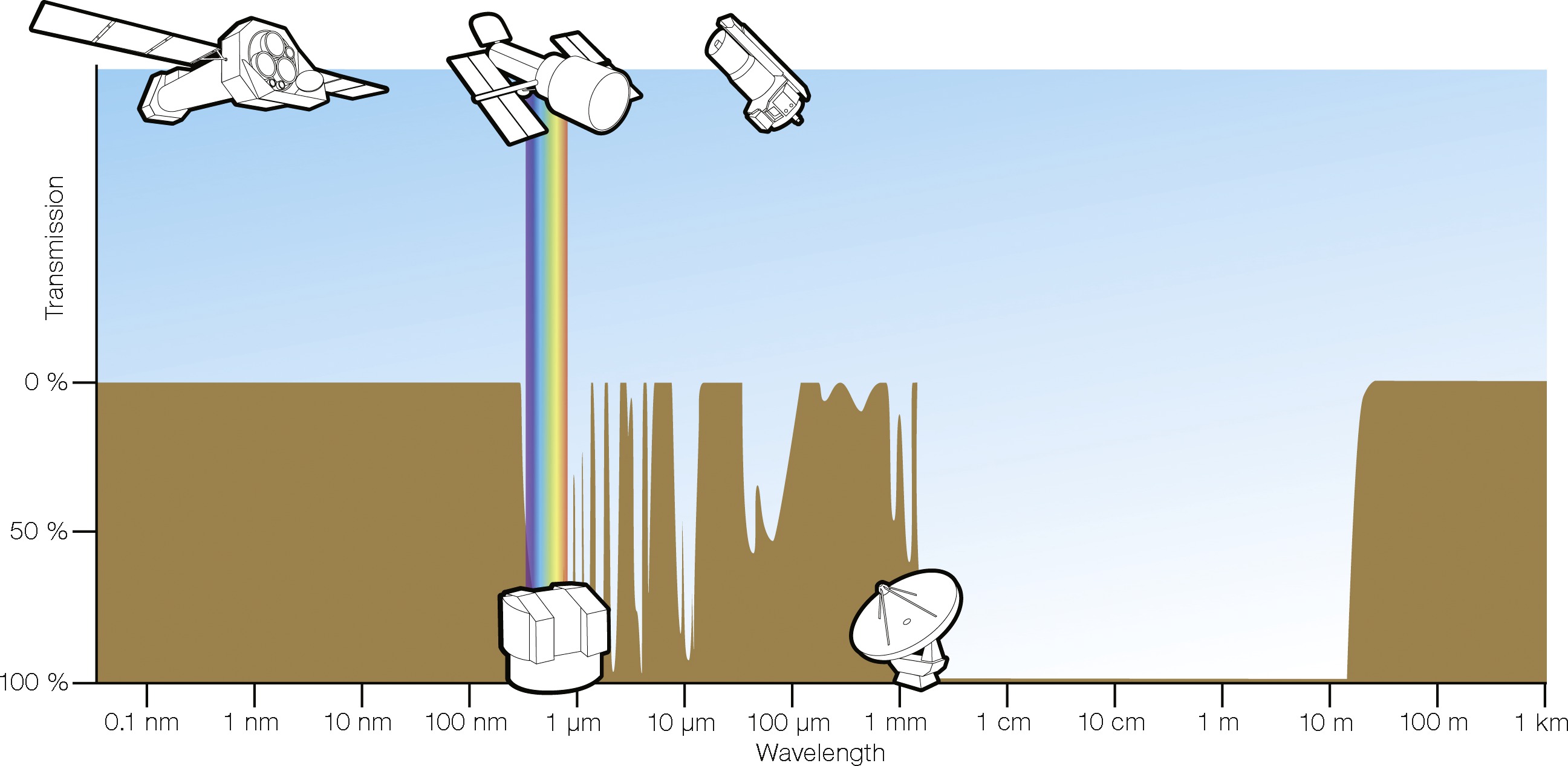
What physical processes limit the atmospheric windows? At the high-frequency end of the radio window, vibrational transitions of atmospheric molecules such as CO, O, and HO have energies comparable with those of mid-infrared photons, so vibrating molecules absorb most extraterrestrial mid-infrared radiation. Lower-energy rotational transitions of atmospheric molecules define the fairly broad transition between the far-infrared band and the high-frequency limit of the radio window at THz. Ground-based radio astronomy is increasingly degraded at frequencies MHz (wavelengths m) by variable ionospheric refraction, and celestial radio waves having frequencies MHz (wavelengths m) are usually reflected back into space by the Earth’s ionosphere. Total internal reflection in the ionosphere makes the Earth look like a mirror from space, like the glass face of an underwater wristwatch viewed obliquely.
Ultraviolet photons have energies close to the binding energies of the outer electrons in atoms, so electronic transitions in atoms account for the high ultraviolet opacity of the atmosphere. Higher-energy electronic and nuclear transitions produce X-ray and gamma-ray absorption. In addition, Rayleigh scattering of sunlight by atmospheric gas molecules and dust particles at visible and ultraviolet wavelengths brightens the sky enough to preclude daytime optical observations of faint objects. Radio wavelengths are much longer than atmospheric dust grains and the Sun is not an overwhelmingly bright radio source, so the radio sky is always dark and many radio observations can be made day or night.
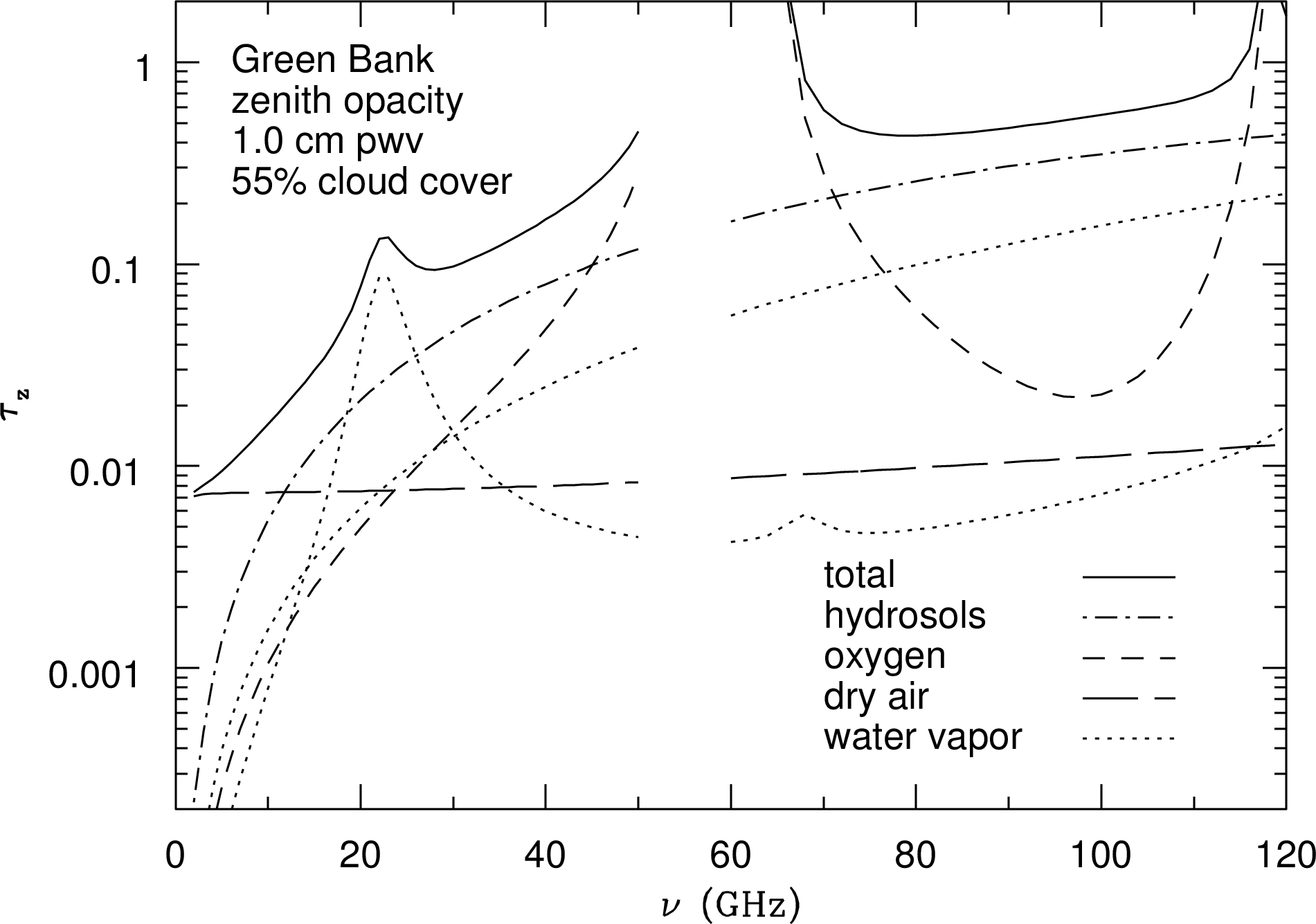
The atmosphere is not perfectly transparent at any radio frequency. Figure 1.2 shows how its zenith (the zenith is the point directly overhead) opacity in Green Bank, WV varies with frequency during a typical summer night with a water-vapor column density of 1 cm, 55% cloud cover, and surface air temperature . The total zenith opacity (solid curve) is the sum of several components [66]:
-
1.
The broadband or continuum opacity of dry air (long dashes) results from viscous damping of the free rotations of nonpolar molecules. It is relatively small () and nearly independent of frequency.
-
2.
Molecular oxygen (O) has no permanent electric dipole moment, but it does have rotational transitions that can absorb radio waves because it has a permanent magnetic dipole moment. The atmospheric-pressure-broadened complex of oxygen spectral lines (short dashes) is quite opaque () and precludes ground-based observations in the frequency range ().
-
3.
Hydrosols are liquid water droplets small enough (radius mm) to remain suspended in clouds. They are much smaller than the wavelength even at 120 GHz ( mm), so their emission and absorption obey the Rayleigh scattering approximation and their opacity (dot-dash curve) is proportional to or .
-
4.
The strong water-vapor spectral line at GHz is pressure broadened to GHz width. The so-called “continuum” opacity of water vapor at radio wavelengths is actually the sum of line-wing opacities from much stronger water lines at infrared wavelengths [107]. In the plotted frequency range, this continuum opacity is also proportional to . Both the line and continuum zenith opacities (dotted curves) are directly proportional to the column density of precipitable water vapor (pwv) along the vertical line of sight through the atmosphere. Conventionally pwv is expressed as a length (e.g., 1 cm) rather than as a true column density (e.g., 1 gm cm), but the two forms are numerically equivalent because the mass density of water is unity in CGS units.
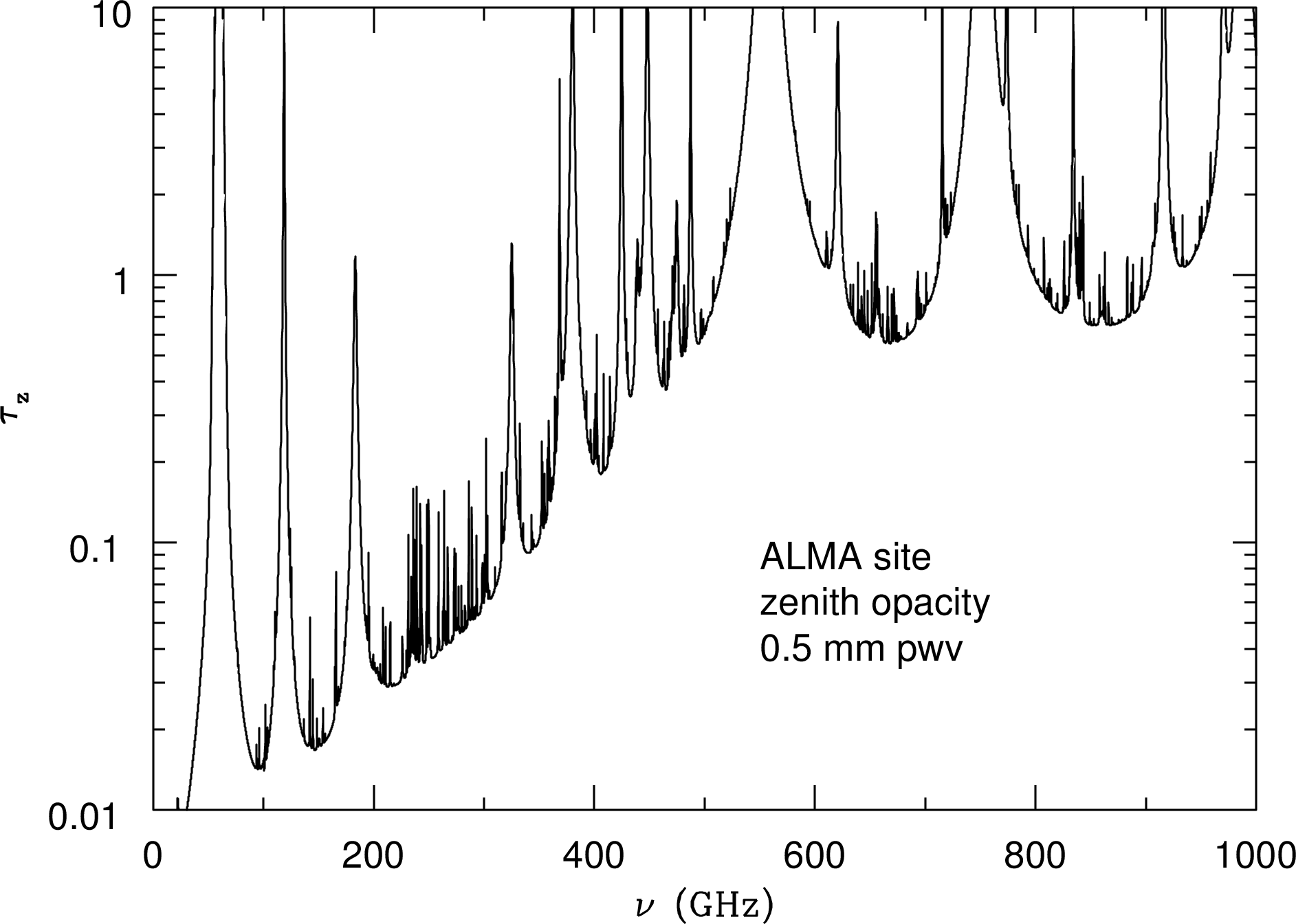
The partially absorbing atmosphere doesn’t just attenuate incoming radio radiation; it also emits radio noise that can seriously degrade the sensitivity of ground-based radio observations. If the atmospheric opacity is , the atmospheric transparency is and emission from the atmosphere at kinetic temperature K adds to the system noise temperature . Radio astronomers use , where Boltzmann’s constant , as a convenient measure of the noise power per unit bandwidth . The system noise temperature is normally much smaller than the atmospheric kinetic temperature, so the added noise from atmospheric emission degrades sensitivity even more than pure absorption alone. For example, emission by water vapor in the warm and humid atmosphere above Green Bank, WV precludes sensitive observations near the water-vapor line at GHz during the summer. Green Bank can be quite cold and dry in the winter, allowing observations at frequencies up to . The very best sites for observing at higher frequencies are exceptionally high and dry. For example, the Atacama Large Millimeter Array (ALMA) shown in Figure 8.5 is located at 5000 m elevation on a desert plain near Cerro Chajnator in Chile, where the typical pwv is mm. Figure 1.3 shows the zenith atmospheric opacity at the ALMA site when pwv mm, for frequencies up to the atmospheric limit.
Finally, the refractive index of water vapor is about 20 times higher at radio than at optical wavelengths because the index of refraction at wavelength is proportional to the cumulative strength of the water-vapor absorption lines at shorter wavelengths, the strongest of which lie in the far-infrared range . Water vapor is not well mixed in the atmosphere, so fluctuations in the column density of water vapor along the line of sight blur the image of a point radio source. The scale height of water vapor in the troposphere is , so the largest fluctuations have transverse dimensions of several km. Consequently point sources seen by all radio telescopes or radio interferometers smaller than a few km in size are blurred by , and this blurring is nearly independent of wavelength for all . The angular size of the “seeing” disk for interferometers much larger than a few km is inversely proportional to the size of the interferometer. In contrast, optical seeing at wavelengths is dominated by the much smaller () turbulent density fluctuations of dry air. It is only a coincidence that the optical seeing disk is also at the best terrestrial sites. For a thorough review of atmospheric and ionospheric propagation effects, see Thompson, Moran, & Swenson [107, Chapter 13].
1.1.3 Astronomy in the Radio Window
Because the radio window is so broad, (1) almost all types of astronomical sources, thermal and nonthermal radiation mechanisms, and propagation phenomena can be observed at radio wavelengths; and (2) a wide variety of radio telescopes and observing techniques are needed to cover the radio window effectively.
The radio window was explored before there were telescopes in space, so early radio astronomy was a science of discovery and serendipity. It revealed a “parallel universe” of unexpected sources not previously seen, or at least not recognized as being different from ordinary stars. Major discoveries of radio astronomy include
-
1.
nonthermal radiation from our Galaxy [87] and many other astronomical sources;
- 2.
-
3.
cosmological evolution of radio galaxies and quasars [99];
-
4.
thermal spectral-line emission from cold interstellar gas atoms, ions, and molecules;
-
5.
maser (the acronym for microwave amplification by stimulated emission of radiation) emission from interstellar molecules [114];
-
6.
coherent continuum emission from stars and pulsars;
-
7.
cosmic microwave background radiation from the hot big bang [81];
-
8.
pulsars and neutron stars [50];
-
9.
indirect but convincing evidence for gravitational radiation [105];
-
10.
the supermassive black hole at the center of our Galaxy; [8]
-
11.
evidence for dark matter in galaxies, deduced from their Hi (neutral hydrogen) rotation curves [93];
-
12.
extrasolar planets [117];
-
13.
strong gravitational lensing [113].
The following items are some of the features of this parallel universe.
-
1.
It is often violent, reflecting high-energy and explosive phenomena in radio galaxies, quasars, supernovae, pulsars, etc., in contrast to the steady light output of most visible stars.
-
2.
Many radio sources are ultimately powered by gravity instead of by nuclear fusion, the principal energy source of visible stars.
-
3.
It is cosmologically distant. Most continuum radio sources are extragalactic, and they have evolved so strongly over cosmic time that most are seen at lookback times comparable with the age of the universe.
-
4.
It can be very cold. The cosmic microwave background dominates the electromagnetic energy of the universe, but its 2.7 K blackbody spectrum is confined to radio and far-infrared wavelengths. Cold interstellar gases emit spectral lines at radio wavelengths.
With the advent of telescopes in space, the entire electromagnetic spectrum has become accessible to astronomers. Many sources discovered by radio astronomers can now be studied in other wavebands, and new objects discovered in other wavebands (e.g., gamma-ray bursters) can now be followed up at radio wavelengths. Radio astronomy is no longer a separate and distinct field; it is one facet of multiwavelength astronomy. Even so, the radio band retains unique astronomical and technical features.
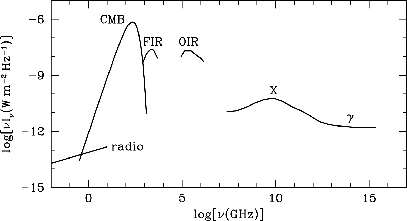
Most of the electromagnetic energy of the universe (Figure 1.4) is in the cosmic microwave background (CMB) radiation left over from the hot big bang. It has a nearly perfect 2.73 K blackbody spectrum peaking at . The strong optical/near-infrared (OIR) peak at (m) is primarily thermal emission from stars plus a smaller contribution of thermal and nonthermal emission from the active galactic nuclei (AGN) in Seyfert galaxies and quasars. Most of the comparably strong cosmic far-infrared (FIR) background peaking at (m) is thermal reemission from interstellar dust that was heated by absorbing about half of that OIR radiation. The cosmic X-ray and gamma-ray backgrounds are mixtures of nonthermal emission (e.g., synchrotron radiation or inverse-Compton scattering) from high-energy particles accelerated by AGN and thermal emission from very hot gas (e.g., gas in clusters of galaxies). By comparison, the relatively faint extragalactic radio-source background (radio) is brighter than the CMB only for . Although many are energetically insignificant, radio sources do trace most phenomena that are detectable in other portions of the electromagnetic spectrum, and modern radio telescopes are sensitive enough to detect them.
1.1.4 What Is Special about Long Wavelengths and Low Frequencies?
Many unique scientific and technical features of radio astronomy result from radio waves occupying the long-wavelength end of the electromagnetic spectrum. At macroscopic wavelengths large groups of charged particles moving together in volumes may produce strong coherent emission, accounting for the astounding radio brightnesses of pulsars at . Dust scattering is negligible because interstellar dust grains are much smaller than radio wavelengths, so the dusty interstellar medium (ISM) is nearly transparent. This allowed radio astronomers to see through the dusty disk of our Galaxy and discover the compact radio source Sgr A [8] powered by the supermassive black hole at its center.
Low frequencies imply low photon energies . Thus radio spectral lines trace extremely low-energy transitions produced by atomic hyperfine splitting (the ubiquitous 21-cm line of neutral hydrogen at GHz generates photons of energy ), the quantized rotation rates of polar molecules such as carbon monoxide in interstellar space, and high-level recombination lines from interstellar atoms.
At radio frequencies, the dimensionless ratio of photon energy to the mean kinetic energy of particles at temperature is very small (). In this limit, the brightness of a blackbody emitter is proportional to , ensuring that nearly every astronomical object is a thermal radio source at some low level. On the negative side, the fact that nearly everything emits radio radiation means radio astronomers must deal with large and fluctuating natural foregrounds of emission from the ground, from the atmosphere, and even from their own antennas and receivers. Also, stimulated emission (negative absorption) becomes comparable with absorption when . This greatly lowers the opacities of radio spectral lines, makes their emission strengths nearly independent of the temperature of the emitting gas, and allows maser emission with only a small population inversion.
In contrast, for cold sources at optical frequencies, where the exponential high-frequency cutoff of the blackbody radiation spectrum ensures that essentially no optical photons are emitted. Cold thermal emitters (e.g., the 2.73 K cosmic microwave background, or interstellar gas at temperatures below 100 K) are completely invisible. For example, a person can be approximated by a 300 K blackbody with a surface area . Such a blackbody emits photons per second at radio frequencies below 10 GHz but only 0.01 photons per second at visible wavelengths .
Free electrons scatter electromagnetic radiation by a process called Thomson scattering or Compton scattering. The Thomson scattering cross section per electron is cm at all frequencies, and sources behind free-electron column densities cm called Compton thick because they are obscured. Radio photons have energies much lower than the eV (electron volt) binding energies of electrons in atoms, so those electrons are not “free” for radio photons, and radio waves can penetrate neutral Compton-thick sources. In contrast, electrons in atoms do not appear bound to X-ray photons with energies, and Compton-thick sources (e.g., “buried quasars” behind clouds of gas and dust) are hidden from X-ray observations.
Radio synchrotron sources live long after their emitting electrons were accelerated to relativistic energies, so they can provide long-lasting archaeological records of past energetic phenomena (e.g., see Figures 8.14 and 8.15). Likewise, neutral hydrogen stripped from colliding galaxies continues emitting at for tens of millions of years (Figures 8.11 and 8.12).
Most plasma effects (scattering, dispersion, Faraday rotation, etc.) have strengths proportional to and are strong enough at low radio frequencies to be useful tools for tracing interstellar electron densities and magnetic field strengths.
1.1.5 Radio Telescopes and Aperture-Synthesis Interferometers
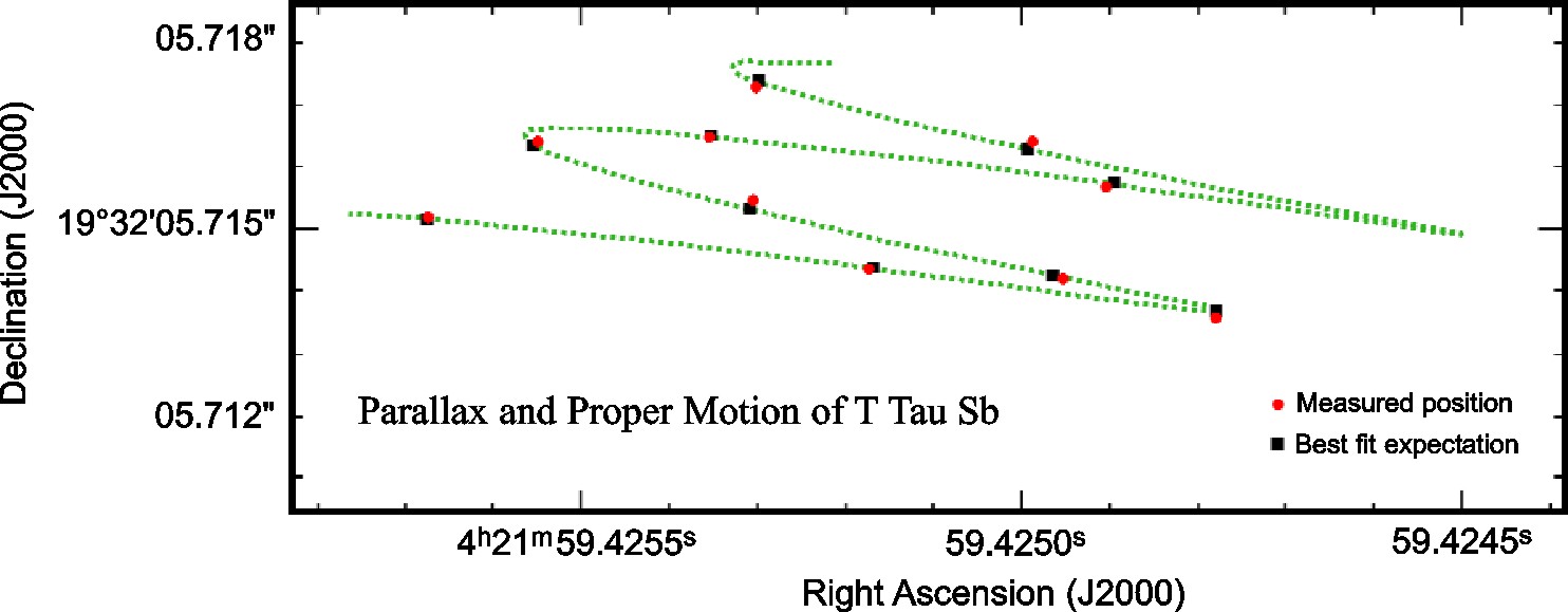
Radio telescopes must have very large aperture diameters to achieve good diffraction-limited angular resolution radians at radio wavelengths. Even the biggest precision radio telescopes (e.g., telescopes with small rms reflector surface errors ) such as the Green Bank Telescope (GBT) (Figure 8.1) with and are limited to . On the other hand, huge multielement interferometers spanning up to km are practical (Figure 1.5). Paradoxically, the finest angular resolution for imaging faint and complex sources is obtainable at the long-wavelength (radio) end of the electromagnetic spectrum. Interferometers also yield extremely accurate astrometry (Figure 1.6) because interferometric positions depend on measuring time delays between telescopes rather than on the mechanical pointing errors of telescopes, and clocks are far more accurate than rulers.
Radio astronomers always measure frequencies directly, while wavelengths are usually measured in the rest of the electromagnetic spectrum. Measuring a frequency has two practical advantages: (1) frequency can be measured more accurately than wavelength because clocks are more accurate than rulers and (2) frequency doesn’t change when radiation passes through a refractive medium, but wavelength does.

Coherent (phase-preserving) amplifiers are required for accurate interferometric imaging of faint extended sources because they allow the signal from each telescope in a multielement interferometer to be amplified before it is split and combined with the signals from the other telescopes, rather than just being divided among the other telescopes. The minimum possible noise temperature of a coherent receiver is owing to quantum noise. Quantum noise is proportional to frequency, so even the best possible coherent amplifiers at visible-light frequencies must have noise temperatures K. Aperture-synthesis interferometers at radio wavelengths provide unparalleled sensitivity, image fidelity, angular resolution, and absolute position accuracy.
1.2 The Discovery of Cosmic Radio Noise
Natural radio emission from our Galaxy was detected serendipitously in 1932 by Karl Guthe Jansky, a physicist working as a radio engineer for Bell Telephone Laboratories. Why hadn’t professional astronomers of that era vigorously pursued radio astronomy and made this discovery first? In part, because they knew too much. They knew that stars are nearly blackbody radiators at visible wavelengths. The spectral brightness at frequency of an ideal blackbody radiator is given by Planck’s law
| (1.1) |
where is the power emitted per unit area per unit frequency per steradian of solid angle by a blackbody, Planck’s constant, frequency in cycles per second, or hertz (so Hz = s), Boltzmann’s constant, the speed of light, and is the absolute temperature (K) of the blackbody.
The subscript in denotes brightness per unit frequency and not brightness as a function of frequency. Likewise, the subscript in denotes brightness per unit wavelength, even if is written as a function of frequency, . Thus but . Both and appear in the astronomical literature, so you have to pay attention to which one is being used. Radio astronomers usually use because electronic spectrometers measure frequencies, but is often appropriate for mechanical spectrometers that measure wavelengths.
At radio frequencies, the dimensionless quantity for most astronomical sources. For example, the temperature of the Sun’s photosphere (the Sun’s visible surface) is K. At GHz Hz, which was near the high-frequency limit of radio technology in 1932,
| (1.2) |
Replacing the exponential denominator in Equation 1.1 by its Taylor-series approximation
| (1.3) |
yields the simple Rayleigh–Jeans approximation
| (1.4) |
or
| (1.5) |
to the blackbody spectrum valid at low frequencies or long wavelengths. The radio emission from a star, which subtends a very small solid angle, would have been too faint to detect. This argument is more-or-less correct; in fact, even the most sensitive modern radio telescopes could not detect the 1 GHz blackbody emission from the photosphere of a star like the Sun if it were moved to the distance pc of the nearest stars (1 parsec (pc) is defined as the distance at which the radius of the Earth’s orbit subtends ).
Nonetheless, Professor Oliver Lodge at Liverpool University tried to detect “long wave” radiation from the Sun in 1894 by “filtering out the ordinary well-known waves by a blackboard” and using a “coherer” of metal filings to detect radio waves. Both “terrestrial sources of disturbance in a city like Liverpool” and an insufficiently sensitive detector foiled this effort [51].
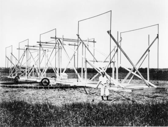
In the 1920s, the Bell Telephone Company offered transatlantic telephone service based on “shortwave” ( m) radio transmissions. Natural radio static was a serious source of interference, so Bell Telephone Laboratories asked their young electrical engineer Karl Jansky to determine its origin. Jansky built the antenna shown in Figure 1.7 to monitor radio static at 20.5 MHz ( m). Its reception pattern was a fan beam (narrow horizontally and broader in the vertical plane) that pointed near the horizon and could be rotated in azimuth—the angle measured from north to east around the horizon. He found that most of the static is produced by lightning strokes in numerous tropical thunderstorms. In addition he discovered a steady “hiss” whose strength rose and fell daily, with a period of 23 hours and 56 minutes. He recognized that this is the length of the sidereal day (the time it takes the Earth to rotate once in the reference frame of the fixed stars), deduced that the hiss must originate somewhere outside the Solar System, and identified the direction to the Galactic center as the source of the strongest emission.
Jansky published his results in the paper “Electrical disturbances of apparently extraterrestrial origin” [57]. His discovery was even announced on the front page of the New York Times, but his employer had no practical interest in understanding the cosmic component of radio static and reassigned Jansky to other projects. Jansky himself believed that the cosmic noise was thermal emission because it produced a steady hiss in headphones that sounded like the hiss generated by hot electrons in vacuum-tube amplifiers. Skeptical astronomers couldn’t understand how such strong (equivalent to the emission from a K blackbody covering most of the inner Galaxy) radio noise was produced, and generally ignored it.
The only person who took a serious interest in Jansky’s discovery was the amateur radio operator and professional radio engineer Grote Reber. He later wrote,
My interest in radio astronomy began after reading the original articles by Karl Jansky. For some years previous I had been an ardent radio amateur and considerable of a DX [long-distance communication] addict, holding the call sign W9GFZ. After contacting over sixty countries and making WAC [Worked All Continents, an amateur-radio award], there did not appear to be any more worlds to conquer. ([88])
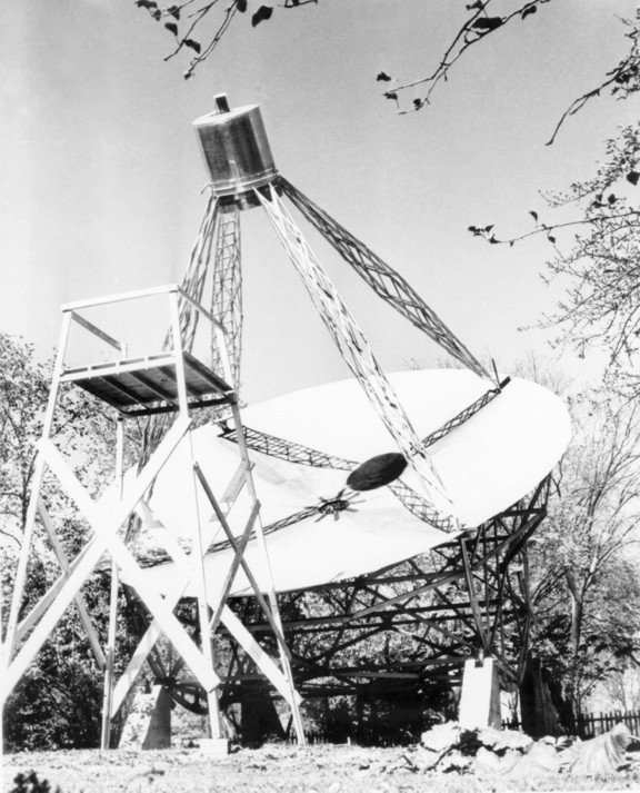
Radio astronomy provided the new worlds to conquer, and radio astronomy became his obsession. He devoted years of his life to building the world’s first radio antenna using a parabolic reflector (Figure 1.8) at his own expense in his back yard in Wheaton, IL and using it to map the Galaxy.
Because Reber also expected to find thermal emission with , he started observing at MHz, the highest technically feasible observing frequency in 1937. When he failed to see anything, he concluded that the radio spectrum of the Galaxy was not Planckian. Next he tried 910 MHz, still with no luck, but “since I am a rather stubborn Dutchman, this had the effect of whetting my appetite for more.” In 1938 he finally succeeded in detecting and mapping (with angular resolution) the Galaxy at 160 MHz, thereby confirming Jansky’s discovery and demonstrating that the radio emission has a distinctly nonthermal spectrum. He observed only at night because automotive ignition interference in Wheaton, IL was too strong during the day. He patiently recorded meter readings by hand once per minute. His results were published in the Astrophysical Journal [87].
Then World War II intervened, hindering astronomical research but stimulating progress in radio and radar technology. Some of the engineers and physicists who developed and used this technology during the war led the rapid scientific development of radio astronomy immediately afterward.
1.3 A Tour of the Radio Universe
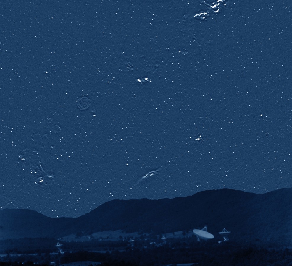
The visible and radio skies reveal distinct “parallel universes” sharing the same space. Most optically bright stars are undetectable at radio wavelengths, and many strong radio sources are optically faint or invisible. Familiar objects like the Sun and planets can appear quite different when seen through the radio and optical windows. The extended radio sources, spread along a band from the lower left to the upper right in Figure 1.9, lie in the outer regions of our Galaxy. The brightest irregularly shaped sources are clouds of hydrogen ionized by luminous young stars. Such stars quickly exhaust their nuclear fuel, collapse, and explode as supernovae; their supernova remnants appear as faint radio rings. Unlike the nearby ( light years) stars visible to the human eye, almost none of the myriad radio “stars” (unresolved radio sources) scattered across the sky are actually stars. Most are extremely luminous radio galaxies or quasars, and their average distance is over light years. Radio waves travel at the speed of light, so distant extragalactic sources appear to us today as they actually were billions (using the “short-scale” definition ) of years ago. Radio galaxies and quasars are beacons carrying information about galaxies and their environs, everywhere in the observable universe and ever since the first galaxies were formed.
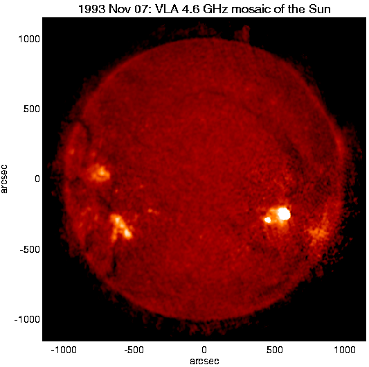
The brightest discrete radio source is the Sun (Figure 1.10), but the Sun is much less dominant than it is in visible light. The radio sky is dark even when the Sun is up because atmospheric molecules and dust particles don’t scatter radio waves whose wavelengths are much larger than these particles. Most radio observations can be made day or night. Clouds are also nearly transparent at wavelengths cm, so long-wavelength radio observations can be made even when the sky is overcast.
The Moon and planets are not detectable by reflected solar radiation at radio wavelengths. However, they all emit thermal radiation, and Jupiter is a strong nonthermal source as well. If the Sun were suddenly switched off, the planets would remain radio sources for a long time, slowly fading as they cooled.
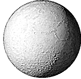
At first glance, the mm radio image of the Moon (Figure 1.11) looks familiar, but it is subtly different from the visible Moon. The darker right edge of the Moon is not being illuminated by the Sun, but it still emits radio waves because it does not cool to absolute zero during the lunar night. The radio emission is not produced at the visible surface; it emerges from a layer about 10 wavelengths thick. As a result, the monthly brightness variations of the Moon decrease as wavelength increases. These wavelength-dependent brightness variations encode information about the thermal conductivity and heat capacity of the rocky and dusty outer layers of the Moon. The craters stand out because their interiors are shielded from sunlight and hence cooler, and also because the steep angles of the crater walls reduce their emissivity (as later explained in Equation 2.47) owing to the Brewster angle effect for dielectric boundaries.
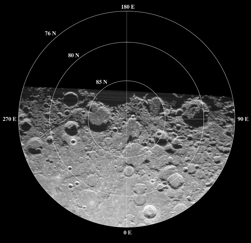
Radar studies of Solar-System objects are active experiments involving artificial radio signals reflected from targets, not just passive observations of natural emission. Planetary radar experiments first determined the rotation period of Venus by penetrating its optically opaque atmosphere, measured a more accurate value for the astronomical unit (the distance between the Earth and the Sun), imaged the topography of the solid planets and moons, and tracked asteroids and comets. Radar images like the one in Figure 1.12 were recently used to search for water ice trapped in cold craters near the lunar poles. For a good introduction to radar astronomy, see the Arecibo radar web page http://www.naic.edu/~pradar/radarpage.html. The principles of radar astronomy are covered in detail by the textbook [36] based on the 1960 MIT summer course in radar astronomy.
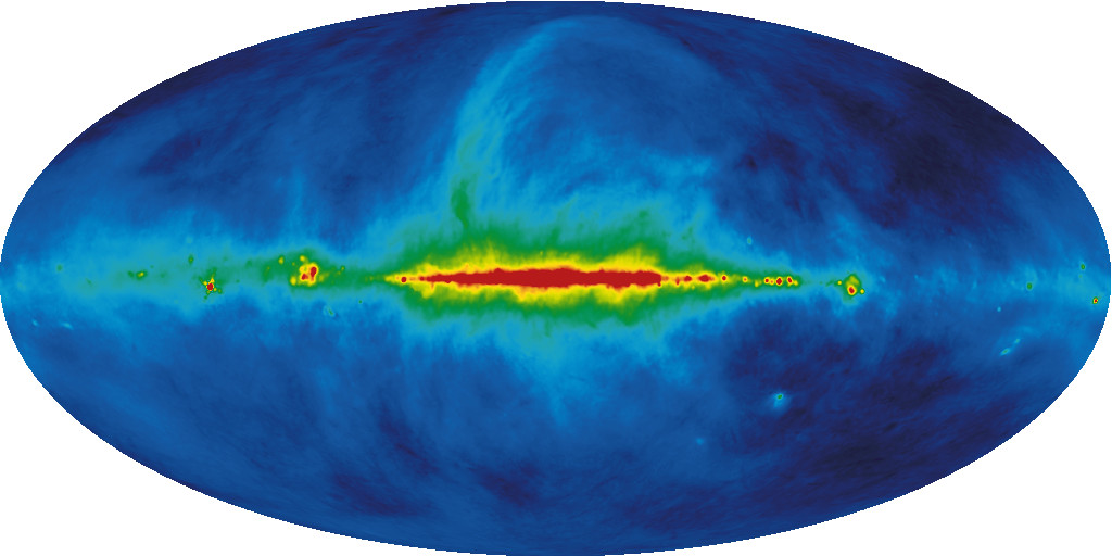
The cosmic static discovered by Karl Jansky is primarily diffuse emission originating in and near the disk of our Galaxy. The distribution of 408 MHz continuum emission displayed in Galactic coordinates (Figure 1.13) is strongest along the Galactic equator, or Galactic latitude , where is the angle from the disk. The brightest radiation comes from near the center of our Galaxy (Galactic longitude ), which is at the center of Figure 1.13.
Galactic interstellar gas emits spectral lines as well as broadband continuum noise. Neutral hydrogen (Hi) gas is ubiquitous in the disk. The brightness of the cm hyperfine line at MHz is proportional to the column density of Hi along the line of sight and is nearly independent of the gas temperature. It is not attenuated by dust absorption, so Hi can be seen throughout the Galaxy and nearby external galaxies (Figure 8.11).
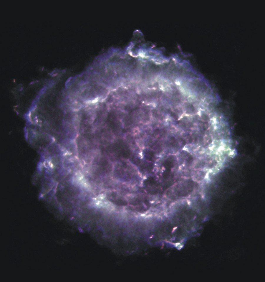
Some of the diffuse continuum emission from our Galaxy can be resolved into discrete sources. Supernova remnants such as Cas A (Figure 1.14) and the Crab Nebula (Figure 8.10), and the relativistic electrons diffused throughout the Galaxy that were accelerated by them, account for about 90% of the GHz continuum emission from our Galaxy. Most of the remaining continuum emission at 1 GHz is thermal emission from Hii regions, hydrogen clouds ionized by UV radiation from extremely massive stars. The nearest large Hii region is the Orion Nebula. Orion’s radio continuum is free–free thermal emission from the hot ionized hydrogen. The dusty nebula is transparent at high radio frequencies, so all of the ionized hydrogen contributes to the radio emission.
Thus massive, short-lived stars are responsible for nearly all of the radio continuum from our Galaxy, and the radio luminosities of most spiral galaxies are proportional to their recent star-formation rates. The nearby “starburst” galaxy M82 (Figure 8.13) has a star-formation rate about 10 times that of our Galaxy and is a correspondingly more luminous radio source. Most galaxies with little or no recent star formation (e.g., elliptical galaxies) are radio quiet. Star-forming galaxies are very common, but their radio sources are not especially luminous, so they account for % of the strongest extragalactic radio sources and somewhat less than half of the cosmic radio-source background.
The strongest extragalactic radio source is the radio Cygnus A (usually shortened to Cyg A) shown in Figure 5.12. The identification of this source in 1954 with a distant (redshift , corresponding to a distance Mpc and a lookback time of about 700 million years) galaxy stunned radio astronomers, who immediately recognized that such luminous radio sources (total radio luminosity W) could be detected almost anywhere in the universe. The angular extent of Cyg A, about 100 arcsec, implies a linear extent kpc, which is much larger than its host galaxy of stars. The energy source is clearly not stars. Gravitational energy released by matter accreting onto a supermassive () black hole in the center of the host galaxy powers this and other luminous extragalactic radio sources. In Figure 8.14 the high-resolution (0.4 arcsec) radio (in red) and optical images of the radio galaxy 3C 348 are superimposed to illustrate their relative sizes.
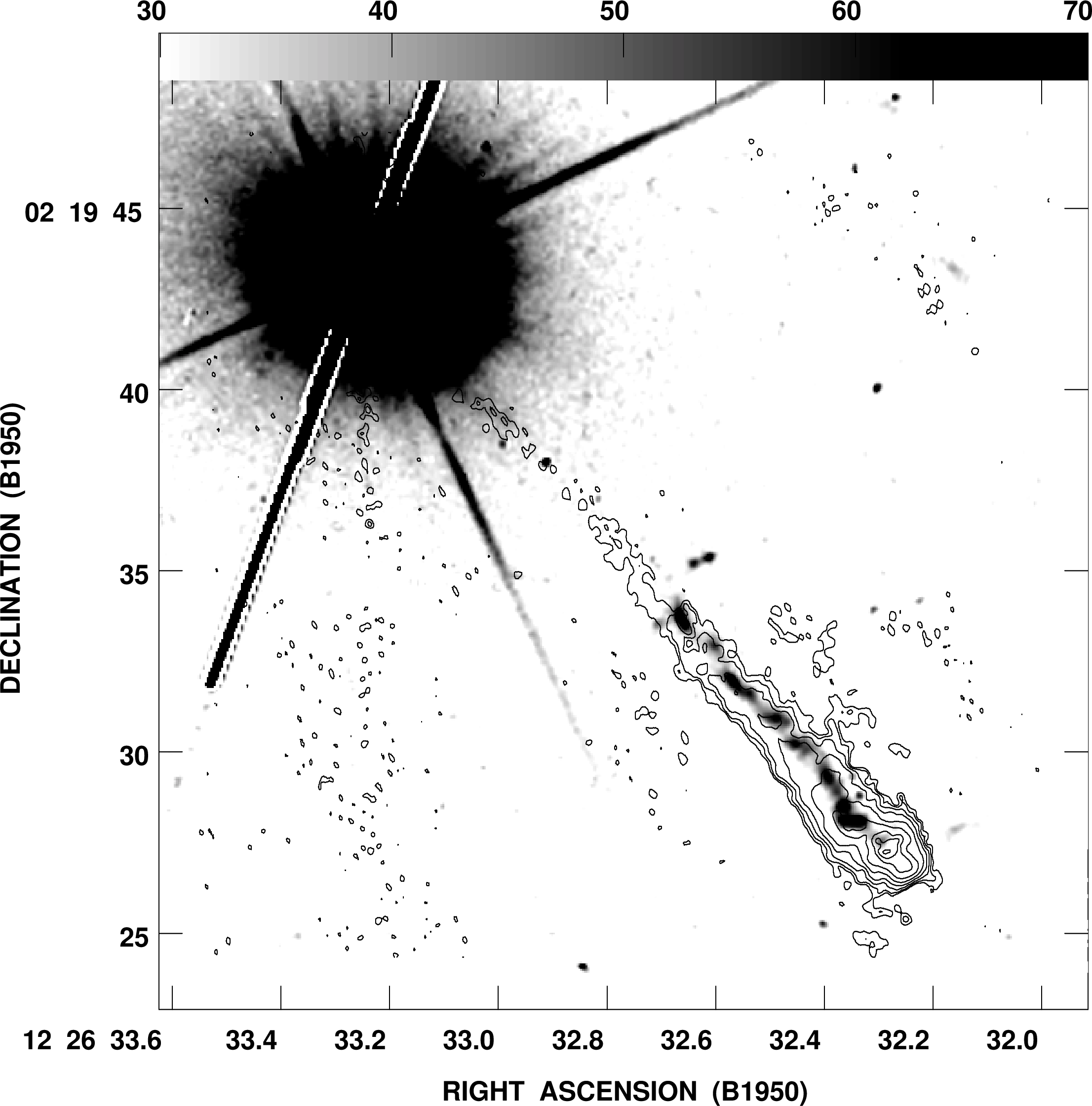
The bright radio source 3C 273 (Figure 1.15) was identified with the first quasar at an even higher redshift, . Such quasars appear to be radio galaxies in an especially active state, when visible light from the region near the black hole overwhelms the starlight from the host galaxy and makes the quasar look like a bright star.
Some exotic phenomena are radio sources but were discovered in other wavelength ranges. Gamma-ray bursts (GRBs) are briefly the most luminous (up to ) discrete sources in the universe, so bright that they were discovered in the 1960s by the VELA nuclear-test monitoring satellites. (For a good history, see the NASA/Swift GRB page.11 1 http://swift.sonoma.edu/about_swift/grbs.html.) Their faint radio afterglows have proven very useful for constraining the energetics and parent populations of GRBs.
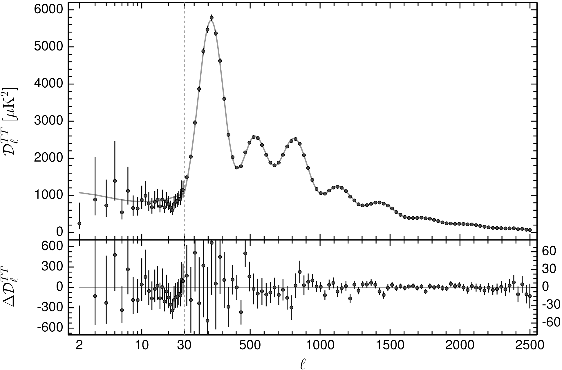
The final stop on any tour of the radio universe is the cosmic microwave background radiation (CMBR), which is thermal radiation from the hot big bang. It fills the universe and is the energetically dominant component of all electromagnetic radiation. We see the surface of last scattering beyond which the universe was ionized and opaque. No more distant radio sources, even if any exist, could be seen. The surface of last scattering is at redshift , so the photons received today were emitted when the universe was only about years old. The CMBR is very nearly isotropic and very nearly a perfect blackbody with K. The Wilkinson Microwave Anisotropy Probe (WMAP), in orbit near the L2 Lagrange point, and the Planck satellite have made all-sky images of the tiny fluctuations in CMBR brightness (Figure 8.16). The angular power spectrum of these fluctuations (Figure 1.16) revealed by the Planck satellite of the European Space Agency (ESA) constrains a host of fundamental cosmological parameters. See the Planck22 2 http://www.cosmos.esa.int/web/planck. and WMAP33 3 http://map.gsfc.nasa.gov/. websites for the most recent results.