Chapter 2 Radiation Fundamentals
2.1 Brightness and Flux Density
Astronomers study an astronomical source by measuring the strength of its radiation as a function of direction on the sky (by mapping or imaging) and frequency (spectroscopy), plus other quantities (time, polarization) to be considered later. Clear and quantitative definitions are needed to describe the strength of radiation and how it varies with direction, frequency, and distance between the source and the observer. The concepts of brightness and flux density are deceptively simple, but they regularly trip up even experienced astronomers. It is very important to understand them clearly because they are so fundamental.
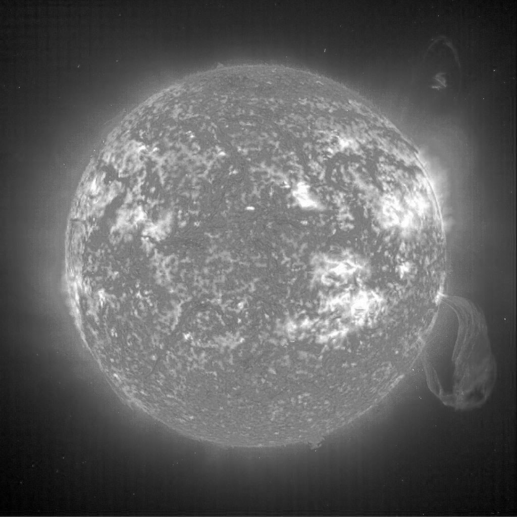
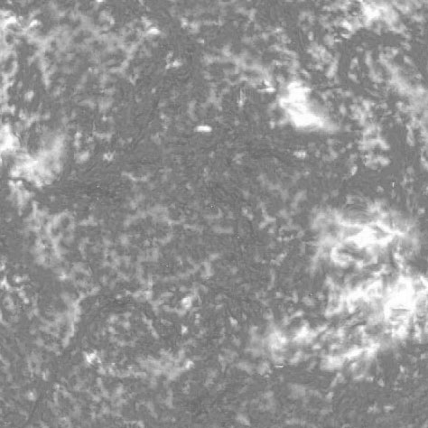
Consider the simplest possible case of radiation traveling from a source through empty space, so there is no absorption (destruction of photons), scattering (changing the direction of photons), or emission (creation of new photons) along the path to an observer. In the ray-optics approximation, radiated energy flows in straight lines. This approximation is valid only for systems much larger than the wavelength of the radiation, a criterion easily met by astronomical sources. You may find it helpful to visualize electromagnetic radiation as a stream of light particles (photons), essentially bullets that travel in straight lines at the speed of light. To motivate the following mathematical definitions, imagine you are looking at the Sun. The “brightness” of the Sun appears to be about the same over most of the Sun’s surface, which looks like a nearly uniform disk even though it is actually a sphere. This means that a photograph of the Sun would be uniformly exposed across the Sun’s disk. It also turns out that the exposure would not change if photographs were made at different distances from the Sun, from points near Mars, the Earth, and Venus, for example (Figure 2.1).
 |
 |
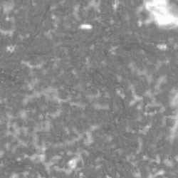 |
The angular size of the Sun depends on the distance between the Sun and the camera, but the number of photons falling on the detector per unit area per unit time per unit solid angle does not. The photo taken from near Venus would not be overexposed, and the one from near Mars would not be underexposed. The total number of solar photons from all directions reaching the camera per unit area per unit time (or the total energy absorbed per unit area per unit time) does decrease with increasing distance, but only because the solid angle subtended by the Sun decreases. Thus we distinguish between the brightness or intensity of the Sun’s radiation, which does not depend on distance, and the apparent flux, which does. Some authors [16, 20] prefer to use brightness for the power per unit area per unit solid angle emitted at the source and specific intensity for the power per unit area per unit solid angle along the path to the detector; others [107, 116] do not distinguish between them. The two are identical if there is no absorption or emission between the source and the detector, and we will use these terms interchangeably.
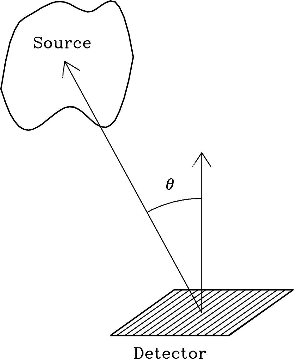
Note also that the number of photons per unit area hitting the detector is proportional to if the normal to the detector is tilted by an angle from the direction of the incoming rays (Figure 2.2). This is just the same projection effect that reduces the amount of water collected by a tilted rain gauge by . Likewise at the source, such as the spherical Sun, the projected area perpendicular to the line of sight is proportional to , where is the angle between the line of sight and the normal to the Sun’s surface.
The total brightness is contributed by photons of all frequencies. The brightness per unit frequency is called the specific intensity (also spectral intensity or spectral brightness). The notation for specific intensity is , where the subscript is used to indicate “per unit frequency.” In the ray-optics approximation, specific intensity can be defined quantitatively in terms of
-
•
= an infinitesimal surface area (e.g., of a detector);
-
•
= the angle between a “ray” of radiation and the normal to the surface;
-
•
= an infinitesimal solid angle measured from the observer’s location.
The surface containing can be any surface, real or imaginary; that is, it could be the physical surface of the detector, the source, or an imaginary surface anywhere along the ray. If energy from within the solid angle flows through the projected area in time and in a narrow frequency band of width , then
| (2.1) |
Power is defined as the flow of energy per unit time, so the corresponding power is
Thus the quantitative definition of specific intensity or spectral brightness is
| (2.2) |
and the MKS units of are .
Radio astronomers almost always measure frequencies, but observers in other wavebands normally measure wavelengths rather than frequencies, so the brightness per unit wavelength
| (2.3) |
is also widely used. The MKS units of are . The relation between the intensity per unit frequency and the intensity per unit wavelength can be derived from the requirement that the power in the frequency interval to must equal the power in the corresponding wavelength interval to :
| (2.4) |
Thus
| (2.5) |
The reasons for specifying the brightness in an infinitesimal frequency range or wavelength range are (1) the detailed spectra of sources carry astrophysically important information, (2) source properties (e.g., opacity) may vary with frequency, and (3) most general theorems about radiation are true for all narrow frequency ranges (e.g., specific intensity is conserved along a ray path in empty space), so they are also true for any wider frequency range. Thus the conservation of specific intensity (Equation 2.7) implies that total intensity defined as
| (2.6) |
is also conserved.
Theorem. Specific intensity is conserved (is constant) along any ray in empty space.
This follows directly from geometry. Let and be two infinitesimal surfaces along a ray of length , as shown in Figure 2.3.
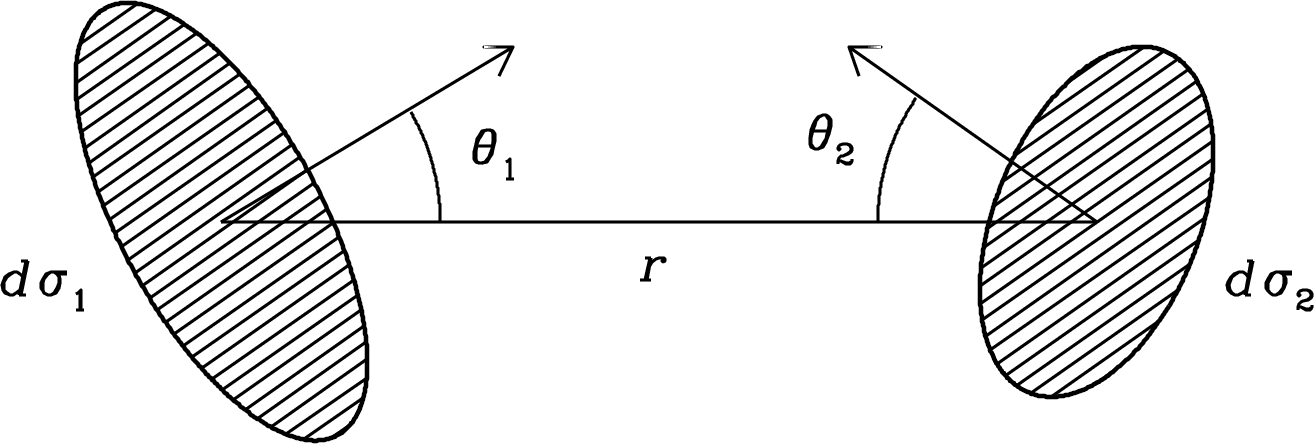
Let rad be the solid angle subtended by as seen from the center of the surface and rad be the solid angle subtended by as seen from the center of the surface . Then
The power in the frequency range to flowing through the area in solid angle is
Likewise
Radiation energy is conserved in free space (where there is no absorption or emission), so and
| (2.7) |
The conservation of specific intensity has two important consequences:
-
1.
Brightness is independent of distance. Thus the camera setting for a good exposure of the Sun would be the same, regardless of whether the photograph was taken close to the Sun (from near Venus, for example) or far away from the Sun (from near Mars, for example), so long as the Sun is resolved in the photograph.
-
2.
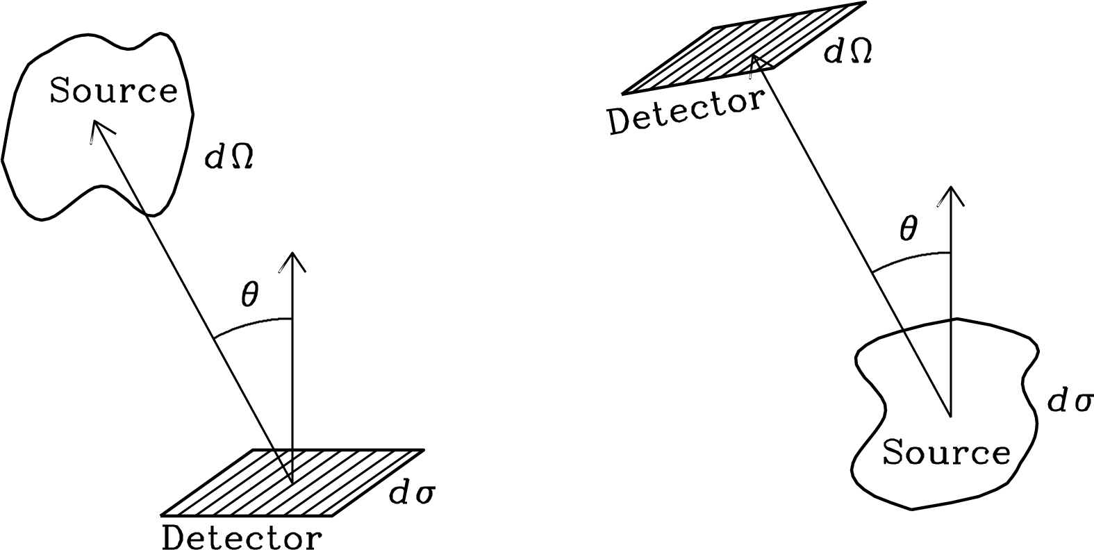
Brightness is the same at the source and at the detector. Thus you can think of brightness in terms of energy flowing out of the source or as energy flowing into the detector (Figure 2.4).
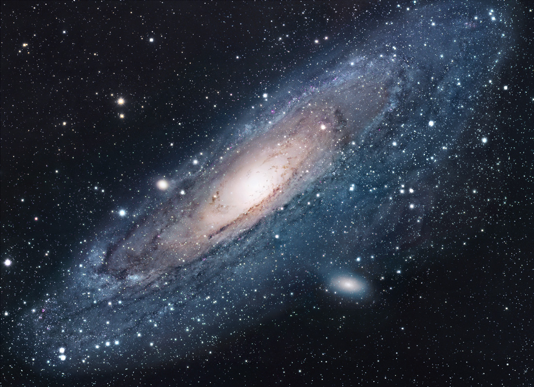
The conservation of brightness applies to any lossless optical system (a system of lenses and mirrors, for example) that can change the direction of a ray. No passive optical system can increase the specific intensity or total intensity of radiation. If you look at the Moon through a large telescope, the Moon will appear bigger (in angular size) but not brighter. Many people are disappointed when they see a large galaxy through a telescope because it looks so dim; they expected to see a brilliantly glowing disk of stars, as in the photograph of Andromeda in Figure 2.5. The difference is not in the telescope; it is in the detector—the photograph appears brighter only because the photograph has accumulated more light over a long exposure time.
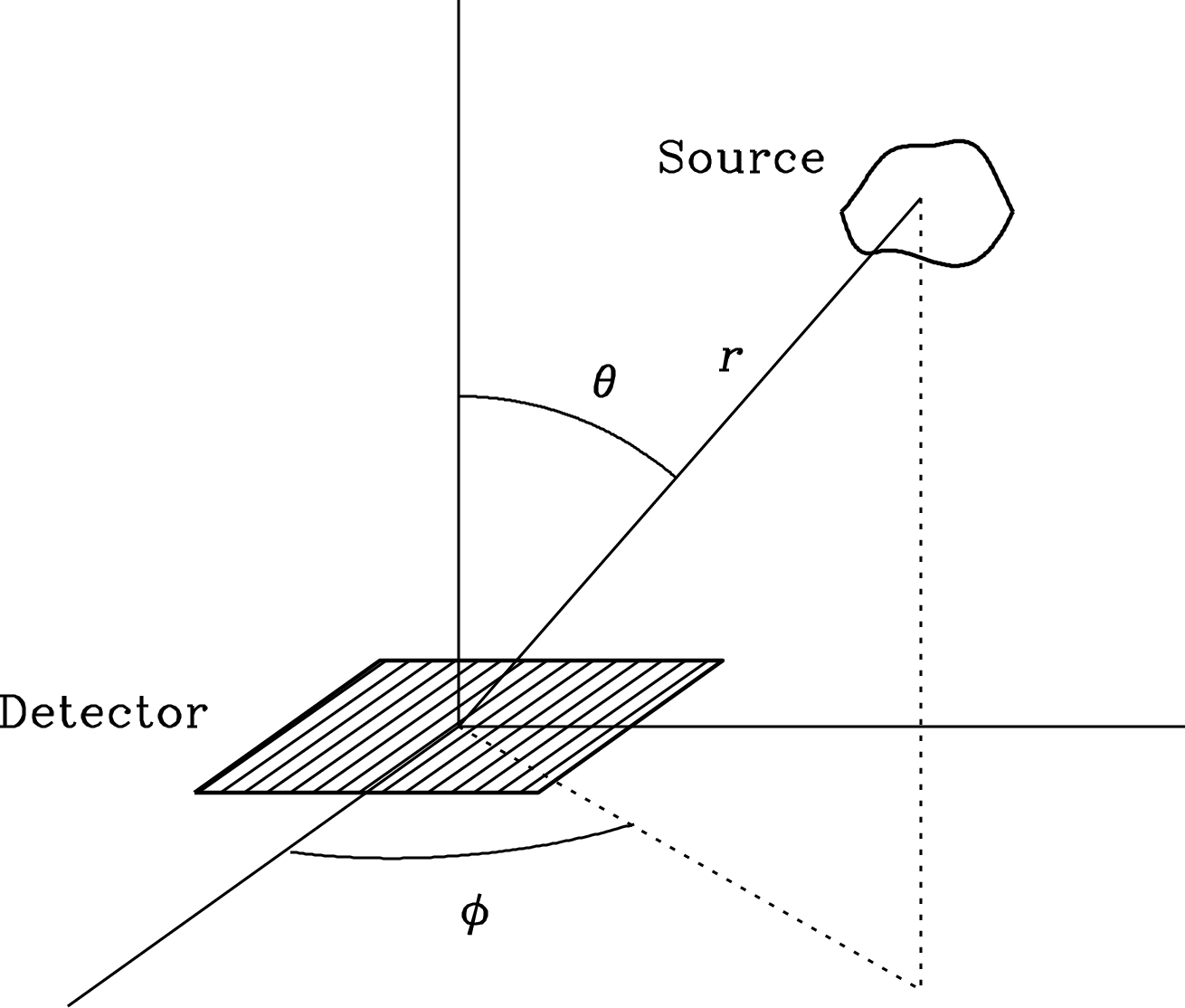
If a source is discrete, meaning that it subtends a well-defined solid angle, the spectral power received by a detector of unit projected area (Figure 2.6) is called the flux density of the source. Equation (2.2) implies
| (2.8) |
so integrating over the solid angle subtended by the source yields
| (2.9) |
If the source angular size is , and the expression for flux density is much simpler:
| (2.10) |
This is usually the case for astronomical sources, and astronomers rarely use flux densities to describe sources so extended that the factor must be retained (e.g., the diffuse emission from our Galaxy).
In practice, when should spectral brightness and when should flux density be used to describe a source? If a source is unresolved, meaning that it is much smaller in angular size than the point-source response of the eye or telescope observing it, its flux density can be measured but its spectral brightness cannot. To the naked eye, the unresolved red giant star Betelgeuse appears to be one of the brightest stars in the sky. Yet calling it a “bright star” is misleading because the total intensity of this relatively cool star is lower than the total intensity of every hotter but more distant star that is scarcely visible to the eye. Betelgeuse appears “brighter” than most other stars only because it subtends a much larger solid angle and therefore its flux is higher. If a source is much larger than the point-source response, its spectral brightness at any position on the source can be measured directly, but its flux density must be calculated by integrating the observed spectral brightnesses over the source solid angle. Consequently, flux densities are normally used to describe only relatively compact sources.
The MKS units of flux density, , are much too big for practical astronomical use, so astronomers use smaller ones:
| (2.11) |
1 millijansky = 1 mJy Jy, and 1 microjansky = 1 Jy Jy. Optical astronomers often express flux densities as AB magnitudes defined in terms of Jy by
| (2.12) |
Unlike brightness, flux density depends on source distance . Because and brightness is conserved, Equation 2.10 implies the inverse square law:
| (2.13) |
The specific intensity or brightness is an intrinsic property of a source, while the flux density of a source also depends on the distance between the source and the observer.
The total flux or flux from a source is the integral over frequency of flux density:
| (2.14) |
Its dimensions are power divided by area, so its MKS units are W m. Total flux is a rarely used quantity in observational radio astronomy, so radio astronomers often delete the subscript from and use the symbol to indicate flux density. This is convenient but potentially confusing. Likewise, the word “flux” is sometimes used as a shorthand for “flux density” in the literature, even though it is formally incorrect.
The spectral luminosity of a source is defined as the total power per unit bandwidth radiated by the source at frequency ; its MKS units are . The area of a sphere of radius is , so the relation between the spectral luminosity and the flux density of an isotropic source radiating in free space is
| (2.15) |
where the distance between the source and the observer is much larger than the dimensions of the source itself. Beware that some radio sources emit anisotropically, relativistically beamed quasars (Section 5.6.1) for example. Unfortunately, Equation 2.15 cannot be used to calculate the total (integrated over ) spectral luminosity of a beamed quasar from a flux-density measurement made from just one direction. Spectral luminosity is an intrinsic property of the source because it does not depend on the distance between the source and the observer—the in Equation. 2.15 cancels the dependence of . The luminosity or total luminosity of a source is defined as the integral over all frequencies of the spectral luminosity:
| (2.16) |
Astronomers sometimes call the bolometric luminosity because a bolometer is a broadband detector that measures the heating power of radiation at all frequencies.
2.2 Radiative Transfer
In free space, the specific intensity of radiation is conserved along a ray:
| (2.17) |
where is the coordinate along the ray between the source and the detector. What happens if there is an intervening medium between and (Figure 2.7)?
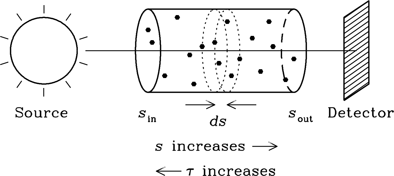
2.2.1 Absorption
Think of the ray as a beam of photons, or light particles, some of which may be absorbed by the medium and vanish. The infinitesimal probability of a photon being absorbed (e.g., by hitting an absorbing particle) in a thin slab of thickness is directly proportional to : , where the constant of proportionality
| (2.18) |
is called the linear absorption coefficient, and its dimension is inverse length. A value means that over some small distance along the ray, m for example, the small fraction of the photons will be absorbed. Why consider such thin layers rather than the whole absorber at once? Only if the layer is thin enough that is infinitesimal does the probability of absorption within the layer increase linearly with thickness so that is a constant independent of . In a layer thick enough to absorb a significant fraction of the photons, fewer photons are absorbed near the far end of the layer simply because fewer photons have survived to be absorbed there, so the probability of absorption increases nonlinearly with thickness.
This simple macroscopic model doesn’t depend on the microscopic physical processes by which photons are absorbed. It is like the ideal gas model, which relates the macroscopic properties of a gas (temperature, pressure, and density) without considering the microscopic details about how individual gas molecules behave.
The fraction of the specific intensity lost to absorption in the infinitesimal distance along the ray is
| (2.19) |
Integrating both sides of Equation 2.19 along the absorbing path gives the output specific intensity as a fraction of the input specific intensity:
| (2.20) | |||
| (2.21) | |||
| (2.22) |
The dimensionless quantity
| (2.23) |
is called the optical depth or opacity of the absorber. Note that . The “backward” direction of the path integration along the line of sight was chosen in Equation 2.23 to make and increasing as you look deeper into an absorber. Thus
| (2.24) |
If , the absorber is said to be optically thin; if , it is optically thick.
2.2.2 Emission
The intervening medium may also emit photons, again by some unspecified microscopic process. In any infinitesimal volume () of thickness and cross section , the probability per unit time that an isotropic source will emit a photon into the solid angle is directly proportional to the volume and solid angle:
| (2.25) |
The emission coefficient is defined so that
| (2.26) |
if there is no absorption. The dimensions of follow from its definition; they are power per unit volume per unit frequency per unit solid angle, and the corresponding MKS units are . Combining the effects of absorption (Equation 2.19) and emission (Equation 2.26) yields the equation of radiative transfer
| (2.27) |
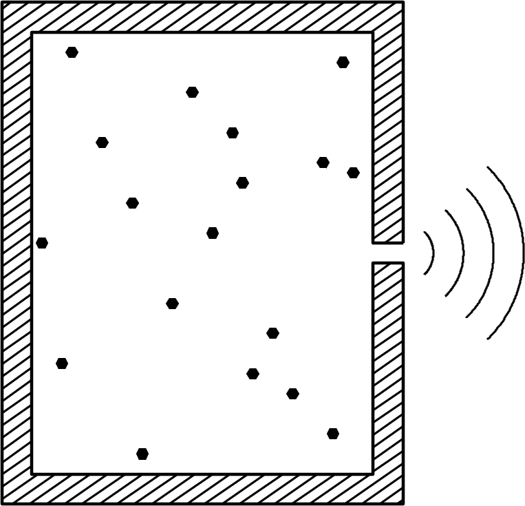
Because the absorption and emission processes have not been specified, and seem to be independent. However, they are not independent in full thermodynamic equilibrium (TE). In TE, matter and radiation are in equilibrium at the same temperature . Cavity radiation from a container bounded by opaque walls pierced by a small hole (Figure 2.8) is equilibrium radiation. The intensity and spectrum of the radiation emerging from the hole is independent of the wall material (e.g., wood painted green, shiny copper, gray concrete, etc.) and any absorbing material (e.g., gas, dust, fog, etc.) that may be inside the cavity.
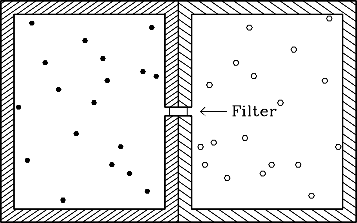
Kirchhoff derived the relation between and in TE using the thought experiment illustrated in Figure 2.9. Two cavities made of different materials and containing different absorbers are connected through a passive (meaning, no energy is needed for it to work) filter transparent only in the narrow frequency range to . In equilibrium at any temperature , radiation can transfer no net power from one cavity to the other, lest one cavity cool down and the other heat up. That would violate the second law of thermodynamics because the two cavities at different temperatures could be used to drive a heat engine.
In (full) thermodynamic equilibrium (TE) at temperature ,
| (2.28) |
where is the spectrum of equilibrium radiation at temperature . The symbol is used because equilibrium cavity radiation is the same as the blackbody radiation for a perfect absorber at temperature , even if it is not in a cavity. Rearranging the equation of radiative transfer (Equation 2.27)
| (2.29) |
yields Kirchhoff’s law for a system in TE:
| (2.30) |
which is valid at any frequency . Equation 2.30 is remarkable because it connects the properties and of any kind of matter to the single universal spectrum of equilibrium radiation. Note also that Kirchhoff’s argument is independent of the shapes of the cavities, so cavity radiation must be isotropic.
Although Kirchhoff’s law was derived for a system in thermodynamic equilibrium, its applicability is not limited to radiation in full thermodynamic equilibrium with its material environment. Kirchhoff’s law also applies whenever the radiating/absorbing material is in thermal equilibrium, in any radiation field. If the emitting/absorbing material is in thermal equilibrium at a well-defined temperature , it is said to be in local thermodynamic equilibrium (LTE) even if it is not in equilibrium with the radiation field. For example, gas molecules in the Earth’s lower atmosphere have a Maxwellian speed distribution (Equation 4.34), so the gas is in LTE. The gas has a well-defined kinetic temperature K measurable with an ordinary thermometer, but it is in a distinctly nonequilibrium radiation field (anisotropic K sunlight during the day, the cold dark sky at night, plus anisotropic emission from the ground).
Kirchhoff’s law applies in LTE as well as in TE. To show this, recall that is independent of the properties of the radiating/absorbing material. In contrast, both and depend only on the materials in the cavity (e.g., whether the walls are made of copper or concrete) and on the temperature of that material; they do not depend on the ambient radiation field or its spectrum.
This generalized version of Kirchhoff’s law is an exceptionally valuable tool for calculating the emission coefficient from the absorption coefficient or vice versa. For example, in Section 4.3 Kirchhoff’s law gives immediately following a calculation of for free–free emission by an Hii region (a cloud of ionized hydrogen) in LTE.
The blackbody spectrum (Equation 2.86) falls exponentially at frequencies above the peak, but only as a power law at lower frequencies (solid curve in Figure 2.20). Kirchhoff’s law is not intuitively obvious from experience because room-temperature ( K) objects in our environment are much too cold () to emit detectable amounts of visible light. A glass of water might absorb 10% of the sunlight passing through it, but we do not see any emitted light because 10% (or even 100%) of the blackbody radiation emitted by a room-temperature object is very nearly zero. One familiar example of Kirchhoff’s law is a charcoal fire with flames and glowing coals. The infrared (heat) radiation from barely glowing black coals in LTE is much more intense than that from the hotter but nearly transparent visible flames, as you can verify by using a shield to cover either the coals or the flames. In contrast, the radio emission implied by Kirchhoff’s law is always significant because when and the blackbody spectrum below the peak falls off only as . This point is illustrated by radio emission and absorption in the Earth’s atmosphere (Section 2.2.3).
2.2.3 Emission and Absorption of Radio Waves in the Earth’s Atmosphere
At radio frequencies higher than GHz, absorption by the Earth’s atmosphere may be large enough to affect the accuracy of flux-density measurements and atmospheric emission can increase noise errors. Radio astronomers can determine the amount of atmospheric absorption by measuring the amount of atmospheric emission as a function of zenith angle, or angle from the vertical, and using Kirchhoff’s law to calculate the zenith opacity of the (roughly isothermal) atmosphere at frequency from its kinetic (thermometer) temperature and its radio brightness. The celestial sky above the atmosphere is much colder () at high frequencies, so the “background” emission above the atmosphere can usually be ignored.
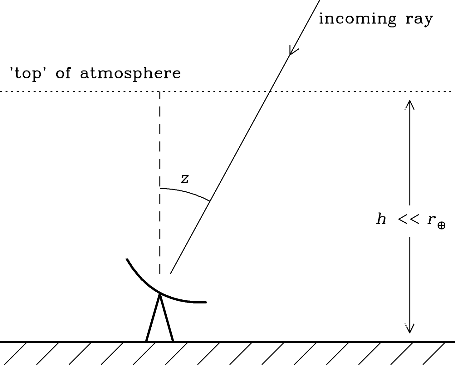
This is done by tilting the radio telescope and measuring as a function of the zenith angle as shown in Figure 2.10. There are two practical complications: (1) The atmospheric signal is noise indistinguishable from other noise sources, especially noise generated in the receiver itself. The output voltage of the receiver is proportional to the sum of these input noise powers. The amount of receiver noise power may not be well known, so only the change in with zenith angle can be measured, not the absolute value of at any zenith angle. (2) The power gain of the receiver system is difficult to calculate from first principles, so most measurements are made relative to some calibration source. For example, the receiver might be calibrated by having the feed look alternately at two absorbing plates with different known temperatures.
Because is directly proportional to in the Rayleigh–Jeans low-frequency approximation
| (2.31) |
radio astronomers often find it convenient to specify the spectral brightness , even if , in terms of the equivalent Rayleigh–Jeans brightness temperature defined by the equation
| (2.32) |
Thus for any ,
| (2.33) |
Equation 2.33 explicitly indicates that can vary with frequency. Brightness temperature is just another way to specify power per unit solid angle per unit bandwidth in terms of the Rayleigh–Jeans approximation. It is convenient because radio telescopes are often calibrated by absorbers or “loads” of known temperature and because the temperature of a radio source is frequently a quantity of physical interest. Beware that brightness temperature is not the same as physical temperature. Nonthermal sources have frequency-dependent brightness temperatures but they do not have well-defined physical temperatures. Thermal sources have brightness temperatures lower than their physical temperatures if they are semitransparent (e.g., the atmosphere) or partially reflecting (e.g., the Moon). Even true blackbody radiators have only in the low-frequency limit .
The observed output from the radio telescope might vary with as shown in Figure 2.11.
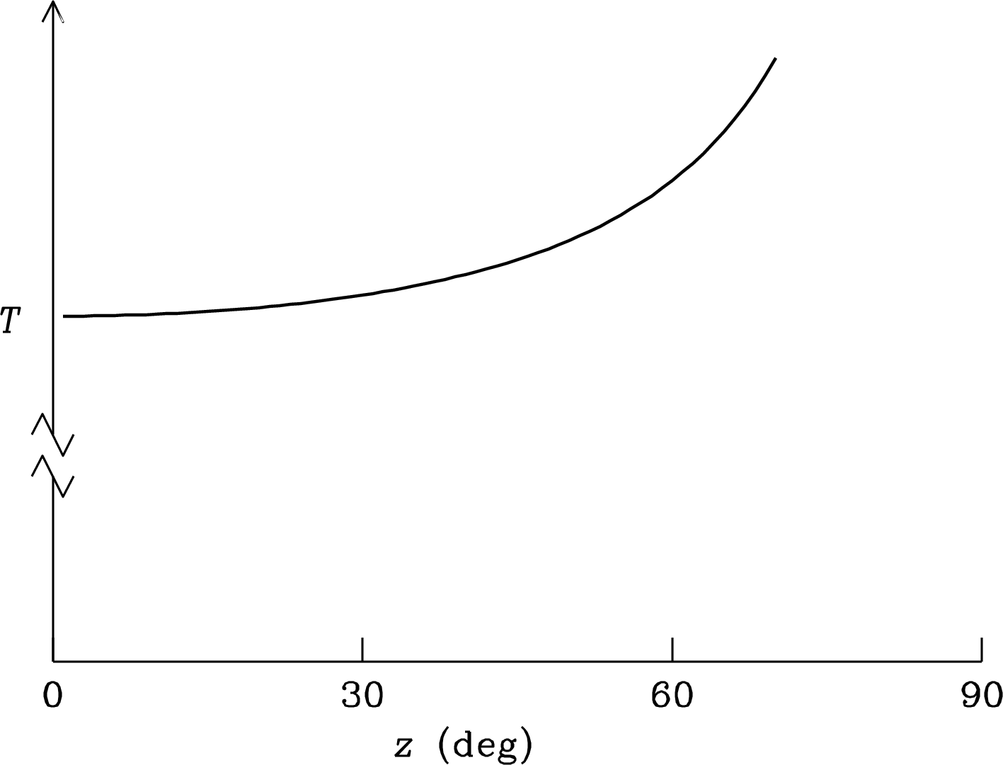
To understand and interpret these observations, start with the radiative transfer equation (2.27),
| (2.34) |
Kirchhoff’s law (Equation 2.30) can eliminate the unknown because the atmosphere is in LTE:
| (2.35) |
where is the kinetic temperature of the atmosphere as measured by an ordinary thermometer. Dividing by yields
| (2.36) |
Multiply both sides of this differential equation by and integrate along the ray in the telescope beam from the top of the atmosphere to the ground. Let be the total optical depth of the atmosphere along the ray at zenith angle . Then
| (2.37) |
Next integrate the left side by parts and take outside the integral (i.e., make the approximation that the atmosphere below altitude is nearly isothermal):
| (2.38) | |||
| (2.39) |
The term can be neglected because the brightness of emission above the atmosphere is small and doesn’t depend on zenith angle at high radio frequencies, so that
| (2.40) |
The path length through a plane-parallel atmosphere is proportional to so at any zenith angle ,
| (2.41) |
where is the zenith opacity of the atmosphere above the radio telescope. Inserting the Rayleigh–Jeans approximation for gives
| (2.42) |
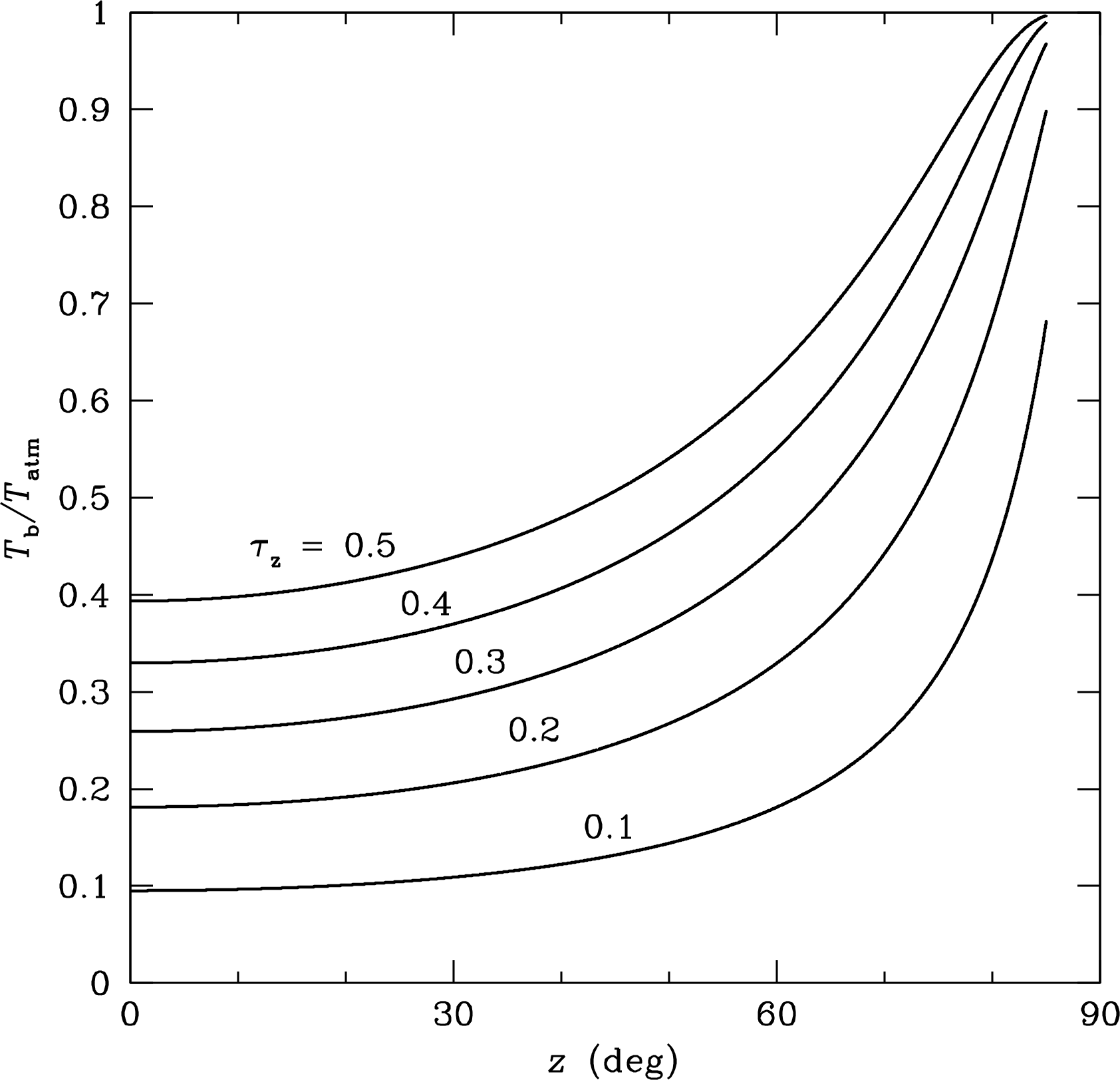
Thus the brightness temperature of the atmospheric emission as a function of zenith angle is
| (2.43) |
The variation of with zenith angle is shown for different zenith opacities in Figure 2.12. By fitting observed data to such curves, radio astronomers can estimate the zenith opacity and correct the measured flux densities of celestial sources for atmospheric absorption.
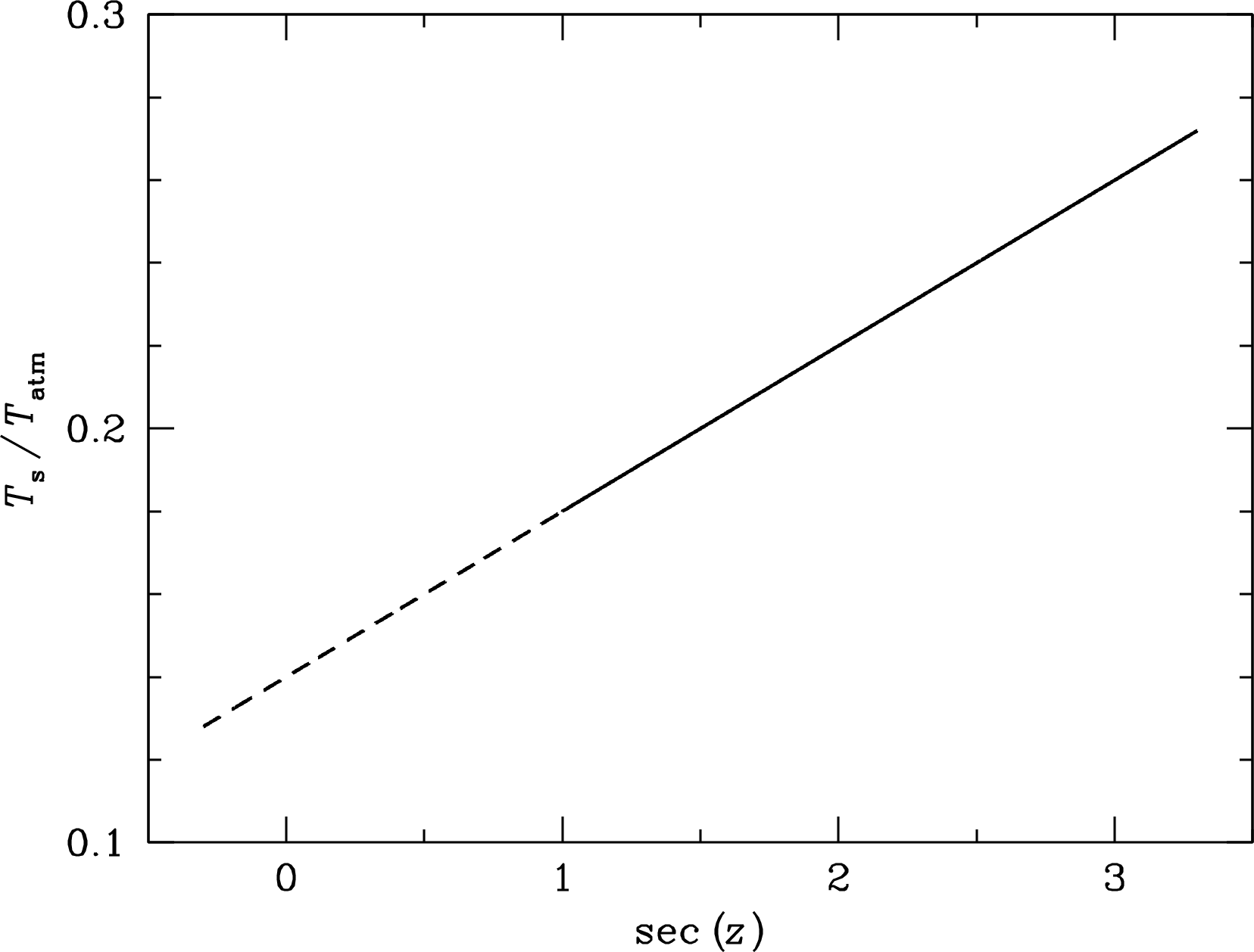
If (1) the zenith opacity is low (), (2) the frequency is high enough () that the radio-source background is weak, and (3) there is little pickup of “spillover” radiation from the ground, then a good approximation to the observed system noise temperature (Equation 3.150) is
| (2.44) |
where is the noise temperature of the receiver alone and is the brightness temperature of the cosmic microwave background. The quantity in square brackets is independent of and is close to the surface air temperature, which can easily be measured with a thermometer. Equation 2.44 implies that the zenith opacity
| (2.45) |
can be read directly from the slope of the linear tipping-curve plot of versus . The solid line in Figure 2.13 shows an example in which . Extrapolating the data to (the geometrically impossible) yields . If , the example implies and thus . Alternatively, if is measured in the laboratory, the tipping curve can be used to determine , the temperature of the cosmic microwave background, corrected for atmospheric emission. This is essentially how Penzias and Wilson [81] discovered the CMB at using the low-spillover Bell Labs horn antenna (Figure 3.19).
2.2.4 Emission, Absorption, and Reflection from an Opaque Body
A body is opaque if its opacity is so high that photons cannot pass through it. The absorption coefficient of an opaque body is the probability that an incident photon of frequency will be absorbed, and the reflection coefficient is the probability that it will be reflected. Thus for a blackbody and for a perfect reflector. Each photon is either absorbed or reflected by any opaque body so
| (2.46) |
The emission coefficient of an opaque body is defined as the ratio of the spectral power it emits per unit area at frequency to that of a blackbody of the same temperature.
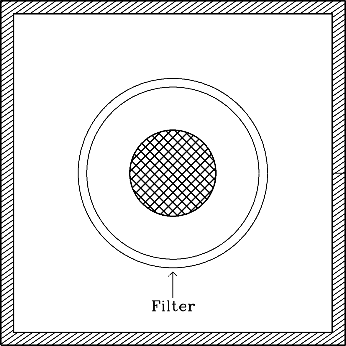
The values of and for any opaque body in local thermodynamic equilibrium are not independent. Imagine an opaque body surrounded by a filter passing frequencies in the range to inside a cavity (Figure 2.14) in thermodynamic equilibrium at some temperature . In equilibrium, the spectral power absorbed by the opaque body must equal the spectral power emitted, so
| (2.47) |
This is Kirchhoff’s law for opaque bodies. It implies that the brightness temperature of an opaque body in LTE at physical temperature is given by
| (2.48) |
Because , then . A perfect reflector () will always have ; that is, it does not emit.
Example. Temperature differences across the GBT reflector (Figure 8.1) caused by differential solar heating can deform the surface and degrade its performance. A special paint that is white at visible wavelengths, black in the mid-infrared, and transparent at radio wavelengths keeps the surface cool and does not harm performance at radio wavelengths by absorbing incoming radio waves or emitting radio noise. The special paint exploits Kirchhoff’s law to perform three separate functions simultaneously: It is opaque and white in the visible portion of the spectrum to reflect sunlight ( K). It is black in the mid-infrared so that the GBT ( K) can cool itself efficiently by reradiation. It is transparent at radio wavelengths so that it neither absorbs incoming radio waves nor emits thermal noise at radio wavelengths.
2.3 Polarization
The instantaneous transverse electric field of a monochromatic electromagnetic wave traveling in the -direction can be projected onto orthogonal - and - (e.g., horizontal and vertical) directions:
| (2.49) |
where is the magnitude of the wave vector pointing in the direction of wave travel,
| (2.50) |
is the angular frequency,
| (2.51) |
is the phase difference between the orthogonal fields and , and
| (2.52) |
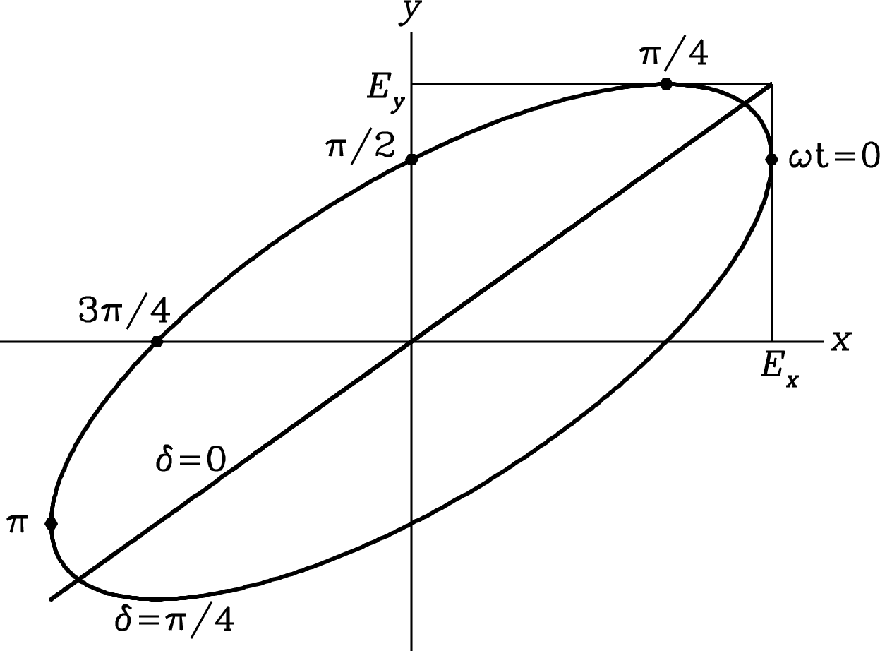
Any time-independent combination of phases and amplitudes yields an elliptically polarized wave (Figure 2.15) whose electric field vector traces out an ellipse in the plane. If the phase difference is zero, the electric field vector does not rotate and the wave is linearly polarized. If and , the electric field vector rotates with angular frequency and traces out a circle; such radiation is said to be circularly polarized. The sign convention for circular polarization used by the Institute of Electrical and Electronics Engineers (IEEE) and by the International Astronomical Union (IAU) is to call the polarization right-handed or left-handed depending on whether the rotation is clockwise () or counterclockwise (), respectively, as viewed from the source toward the observer. An observer looking toward the source sees the electric-field vector from right-handed polarization rotating counterclockwise, as shown by the different time samples in Figure 2.15. Beware that some optics textbooks use the opposite sign convention.
The radiation from astronomical sources is wideband noise whose electric field vector varies rapidly and randomly in amplitude and direction. If radiation in a unit frequency range is averaged over timescales , its average polarization can be characterized by the four Stokes parameters,
| (2.53) | ||||
| (2.54) | ||||
| (2.55) | ||||
| (2.56) |
where the brackets indicate time averages, is the radiation resistance of free space (Equation 3.29), and is the total flux density, regardless of polarization. The polarized flux density is
| (2.57) |
and the degree of polarization is defined as
| (2.58) |
If and have equal amplitudes and their phases are completely uncorrelated, then , , , and the wave is said to be unpolarized. For example, blackbody radiation is unpolarized. An antenna sensitive only to one polarization (e.g., a dipole antenna oriented so it is sensitive only to the component of linear polarization or a helical antenna sensitive only to the left-handed component of circular polarization) will detect only half the power radiated by an unpolarized source. Two orthogonally polarized antennas (e.g., dipoles aligned in the - and -directions or left-handed and right-handed helical antennas) are needed to collect all of the unpolarized power.
Many astronomical sources are partially polarized with . The quantity measures the linearly polarized component of flux, and the ratio depends on the linear polarization position angle. The circularly polarized flux is given by , with indicating right-handed and indicating left-handed circular polarization.
2.4 Blackbody Radiation
A perfect absorber has at all frequencies and is called a blackbody. Kirchhoff’s law (Equation 2.47) requires that every blackbody has emission coefficient at all frequencies as well, so the radiated spectrum of any blackbody at temperature is the same as the spectrum of radiation in thermodynamic equilibrium inside a cavity of temperature , even if the interior walls of the cavity are not black. Thus the intensity and spectrum of blackbody radiation depend only on the temperature of the blackbody or cavity. The most fundamental feature of blackbody radiation is that it is equilibrium radiation; the only reason for discussing cavity radiation is that the cavity traps radiation long enough for it to come into equilibrium. The radiation escaping from a small hole in the cavity is also blackbody radiation because radiation entering the hole from the outside has almost no chance of escaping. A small hole in the side of a very cold cavity looks black. The energy density and brightness spectrum of equilibrium radiation will be derived in Sections 2.4.1 and 2.4.2, even though it will be called blackbody radiation.
The same is true for the electrical noise generated by a warm resistor, a device that completely absorbs electrical energy, and which plays an important role in radio astronomy. The standard derivations of the Rayleigh–Jeans and Planck radiation equations are worth repeating because blackbody radiation is so fundamental and because their one-dimensional analogs yield the spectrum of electrical noise generated by a resistor in equilibrium at temperature .
2.4.1 The Rayleigh–Jeans Approximation
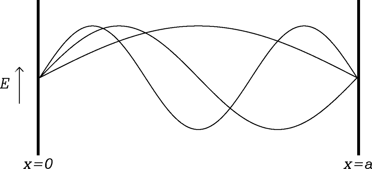
Consider a large (side length , where is the longest wavelength of interest) cubical cavity filled with radiation in thermodynamic equilibrium. The purpose of the cavity is to generate radiation and to confine the radiation long enough for it to reach equilibrium. The radiation must be generated by thermal accelerations of charged particles in the walls of any cavity with . The walls have must have nonzero conductivity because walls of zero conductivity would be transparent—they would generate no currents in response to the electric fields of incoming radiation and the radiation would simply escape. The equilibrium radiation is otherwise independent of the wall material. For walls having nonzero conductivity, the transverse electric field strength at the walls is in equilibrium because fields with induce currents in the walls and lose energy. Only those standing waves with at the walls will persist after some time .
All possible standing-wave modes (a mode is a field pattern that oscillates sinusoidally with a fixed frequency and phase) in the cavity can be enumerated. For example, consider all standing waves whose wave vectors point in the -direction (Figure 2.16). The boundary conditions at and at mean that only those waves having the discrete wavelengths
| (2.59) |
can have nonzero amplitudes. They all satisfy
| (2.60) |
where , 2, 3, Likewise,
| (2.61) |
for wave vectors pointing in the - and -directions, respectively.
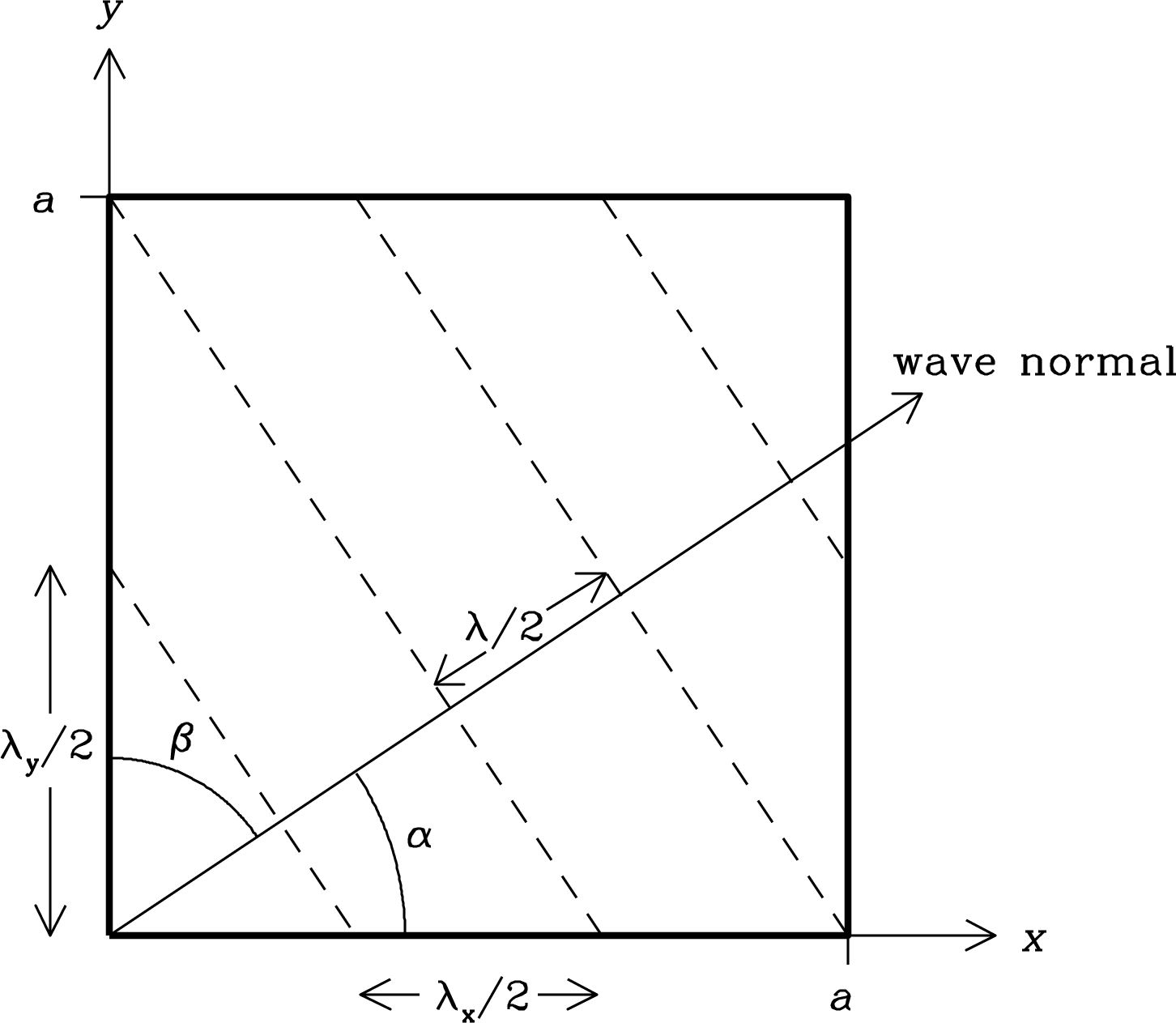
What about a wave vector pointing in some arbitrary direction? Let be the angles between the wave vector and the -, -, -axes, respectively. From Figure 2.18 it is clear that
| (2.62) |
where is the wavelength measured in the direction of the wave vector and is the component of projected onto the -axis. Thus
| (2.63) |
Notice that ; it is divided by , not multiplied by . Simultaneously, the standing waves must also satisfy
| (2.64) |
Equations 2.60 through 2.64 imply that standing waves of all orientations must satisfy
| (2.65) |
| (2.66) |
Squaring and summing the three parts of Equation 2.66 gives
| (2.67) |
The Pythagorean theorem implies so all standing waves must satisfy
| (2.68) |
The permitted frequencies of the standing waves are
| (2.69) |
for all positive integers , , and .
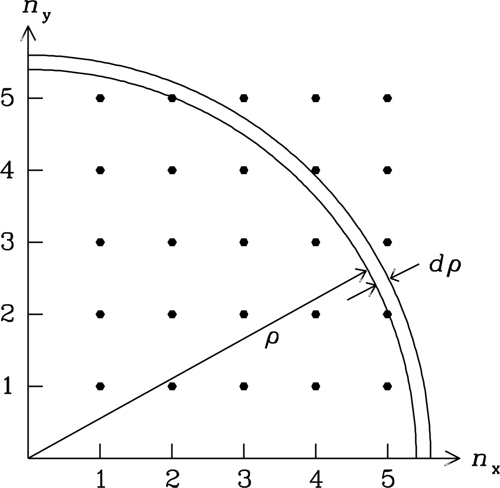
The permitted standing waves can be represented as a lattice in the positive octant of the space whose axes are , , and (Figure 2.18). Each point of the lattice represents one possible mode of equilibrium cavity radiation. The space density of points in this lattice is unity, so the average number of points in any volume equals that volume.
Let be the radial coordinate in -space. Then
| (2.70) |
and
| (2.71) |
The number of independent modes having frequencies in the range to equals the volume of the spherical octant shell between and , multiplied by 2 to account for the two independent orthogonal polarizations (Section 2.3) of electromagnetic waves:
| (2.72) |
Classically, each radiation mode can have any energy . In thermodynamic equilibrium at temperature , the probability that any mode has energy is given by the continuous Boltzmann probability distribution
| (2.73) |
Then the average energy per mode is
| (2.74) |
Thus each mode has the same average energy . The spectral energy density of cavity radiation at frequency is the total energy of all modes (Equation 2.72) at that frequency divided by the volume of the cavity:
| (2.75) |
The spectral energy density of radiation (blackbody or not) is spectral energy per unit volume. It equals the total flow of spectral power per unit area divided by the flow speed :
| (2.76) |
Calling the specific intensity of blackbody radiation and making use of the fact the blackbody radiation is isotropic yields, for blackbody radiation,
| (2.77) |
Combining Equations 2.75 and 2.77 gives
| (2.78) |
Solving for yields the Rayleigh–Jeans approximation for the spectral brightness of blackbody radiation
| (2.79) |
that is valid only in the low-frequency limit .
Notice that
-
1.
the spectral brightness is proportional to frequency squared because the volume of a spherical shell in three dimensions is proportional to frequency squared;
-
2.
all modes have , the classical assumption that breaks down at high frequencies;
-
3.
the Rayleigh–Jeans approximation implies that diverges at high ; this is called the ultraviolet catastrophe;
-
4.
is independent of direction; blackbody radiation is isotropic;
-
5.
blackbody radiation is unpolarized; you can show this with a thought experiment involving two cavities connected by a passive polarizing filter, as in Figure 2.9;
-
6.
this result derived for a cubical cavity applies to equilibrium radiation in a cavity of any shape or (large) size, which you can demonstrate by a thought experiment in which a cubical cavity is connected through a small filter window to the other cavity.
2.4.2 The Planck Radiation Law
The only flaw in the derivation of the Rayleigh–Jeans approximation is the classical assumption that each radiation mode can have any energy . To eliminate the ultraviolet catastrophe, Planck postulated that the possible mode energies are not continuously distributed, but rather they are quantized and must satisfy the new constraint
| (2.80) |
where erg s is Planck’s constant and is the number of photons, or discrete particles of light each having energy
| (2.81) |
Then
| (2.82) |
and the average energy per mode is calculated by summing over only the discrete energies permitted instead of integrating over all energies. Planck’s quantized replacement for Equation 2.74 is
| (2.83) |
Planck’s sum is evaluated in Appendix B.1; it is
| (2.84) |
The quantity is the classical mean energy per mode, and the quantity in square brackets is the quantum correction factor. In the limit the quantum correction factor is unity, but in the limit it falls exponentially to zero. That is, the high-frequency or “ultraviolet” modes may contain few or even zero photons, thereby avoiding the “ultraviolet catastrophe.”
Thus the correct blackbody radiation law becomes
| (2.85) |
where the first factor is the Rayleigh–Jeans approximation and the quantity in square brackets is the quantum correction factor. Planck’s equation for the spectral brightness of blackbody radiation is usually written in the simpler form
| (2.86) |
The corresponding brightness per unit wavelength follows from Equation 2.5; it can be written either as a function of frequency:
| (2.87) |
or as a function of wavelength:
| (2.88) |
Integrating Planck’s law over all frequencies (see Appendix B.2) gives the Stefan–Boltzmann law specifying a finite integrated brightness for a blackbody radiator at temperature :
| (2.89) |
The quantity
| (2.90) |
is called the Stefan–Boltzmann constant and is also derived in Appendix B.2. The unit sr is dimensionless because solid angle has dimensions angle = (length/length). A dimensionless unit can be inserted or deleted without changing the dimensions of an equation—hence the parentheses around sr in Equation 2.90. For clarity it should be used where appropriate. For example, it is needed in the blackbody brightness (erg cm s K sr) Equation 2.89 but not in the radiation energy density (erg cm) Equation 2.93 or in the flux (erg cm s K) Equation 2.111.
For isotropic radiation, the spectral energy density (Equation 2.76) is simply
| (2.91) |
so the total radiation energy density
| (2.92) |
of blackbody radiation is
| (2.93) |
where the quantity
| (2.94) |
is called the radiation constant.
In any narrow frequency range, the number density of photons is their spectral energy density divided by the energy per photon, . The total photon number density is
| (2.95) |
The photon number density of blackbody radiation at temperature is
| (2.96) | ||||
| (2.97) | ||||
| (2.98) |
where the integral
| (2.99) |
is evaluated in Appendix B.2. Numerically, the photon number density of blackbody radiation is
| (2.100) |
The mean photon energy of blackbody radiation is
| (2.101) |
The frequency corresponding to this mean photon energy is
| (2.102) |
It is close to the frequency at which , the brightness per unit frequency of a blackbody, is maximum. Setting
| (2.103) |
yields
| (2.104) |
The wavelength at which
| (2.105) |
maximizes , the brightness per unit wavelength of a blackbody. It is
| (2.106) |
Equation 2.106 is the familiar form of Wien’s displacement law used by optical astronomers, whose spectrometers measure wavelengths instead of frequencies. Note that the peak frequency is much higher than .
The power emitted per unit area per unit frequency by any opaque isotropic radiator of brightness is the spectral flux density
| (2.107) |
where the integration covers the hemisphere above the unit area:
| (2.108) |
| (2.109) |
For a blackbody at temperature , the spectral flux density is
| (2.110) |
The corresponding total power per unit area integrated over all frequencies is
| (2.111) |
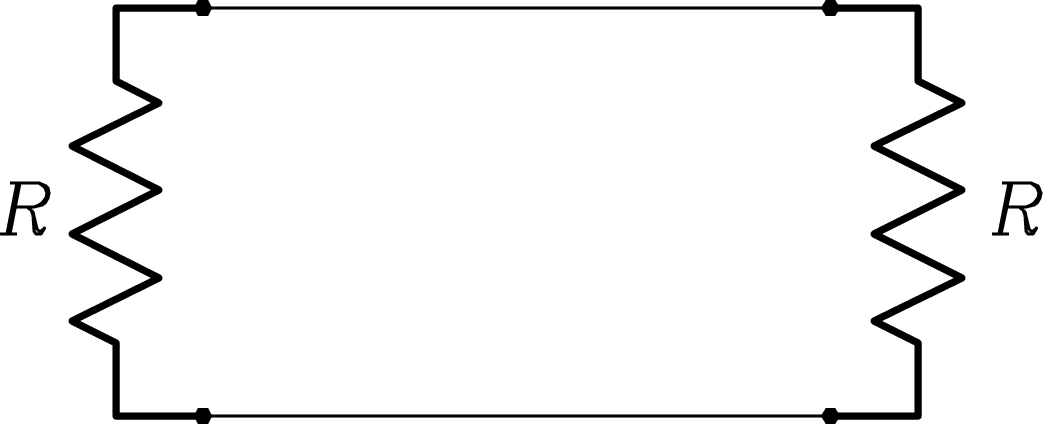
2.5 Noise Generated by a Warm Resistor
A resistor is a passive electronic component that absorbs the electrical power applied to it and converts that power into heat; it is the “blackbody” of electronic circuits. Just as motions of charged particles in the walls of a warm cavity generate photons, motions of charged particles in a resistor at any temperature K generate electrical noise. The frequency spectrum of this noise depends only on the temperature of an ideal resistor and is independent of the material in the resistor.
An antenna is a passive device that converts electromagnetic radiation into electrical currents in wires (when it is used as a receiving antenna) or vice versa (when it is used as a transmitting antenna). The noise generated by a resistor is indistinguishable from the noise coming from a receiving antenna surrounded by blackbody radiation of the same temperature. Warm resistors are useful in radio astronomy as standards for calibrating antennas and receivers, so the noise power per unit bandwidth received by a radio telescope is often described in terms of the Rayleigh–Jeans antenna temperature. The antenna temperature of a receiving antenna is defined as the temperature of an ideal resistor that would generate the same Rayleigh–Jeans noise power per unit bandwidth as appears at the antenna output. Like brightness temperature, antenna temperature is not a physical temperature. The sensitivity and gain of a radio receiver can be calibrated by connecting its input alternately to hot and cold resistors (sometimes called hot and cold “loads”) having known temperatures, and the amount of noise generated in a radiometer (a radio receiver that measures noise power) can be described by the radiometer noise temperature, the temperature of a resistor at the input of an imaginary noiseless radiometer having the same gain as the actual receiver that would generate the same noise power output. Like brightness temperature, radiometer noise temperature is not a physical temperature.
The derivation of the electrical power per unit bandwidth generated by current in a resistor is the one-dimensional analog of the the three-dimensional derivation of the blackbody spectrum [75, 9]. At low radio frequencies, and the Rayleigh–Jeans approximation is accurate. Recall that the Rayleigh–Jeans derivation of starts with a large cube of side length containing standing waves of thermal radiation. The classical average energy in each standing-wave mode is , and the number of modes with frequency to is proportional to , so .
Consider two identical resistors at temperature connected by a lossless transmission line (e.g., a pair of parallel wires) of length much larger than the longest wavelength of interest (Figure 2.20). Standing waves on the line must satisfy
| (2.112) |
where is the wavelength. Electrical signals do not travel at exactly the speed of light on a transmission line, but at some slightly lower velocity so and
| (2.113) |
For , the number of modes per unit frequency is
| (2.114) |
The classical Boltzmann law says that each mode has average energy in equilibrium, so the average energy per unit frequency in the transmission line is
| (2.115) |
This energy takes a time to flow from one end of the transmission line to the other, so the classical power (energy per unit time) per unit frequency flowing on the transmission line is
| (2.116) |
independent of . Thus the total spectral power generated by the two identical resistors must be and, by symmetry, the spectral power generated by each resistor is
| (2.117) |
in the limit . This equation is called the Nyquist approximation and is the electrical equivalent of the Rayleigh–Jeans equation for radiation. Because the “space” of the transmission line has only one dimension instead of three, instead of . The dimensions of are power per unit frequency (e.g., W Hz) and the dimensions of are energy (e.g., joules), which appear to be different at first glance. However, Hz = s, so power per unit frequency W Hz = W s = joule also has dimensions of energy. The latter is simpler, but the former is used because it is conceptually more appropriate for noise power per unit bandwidth.
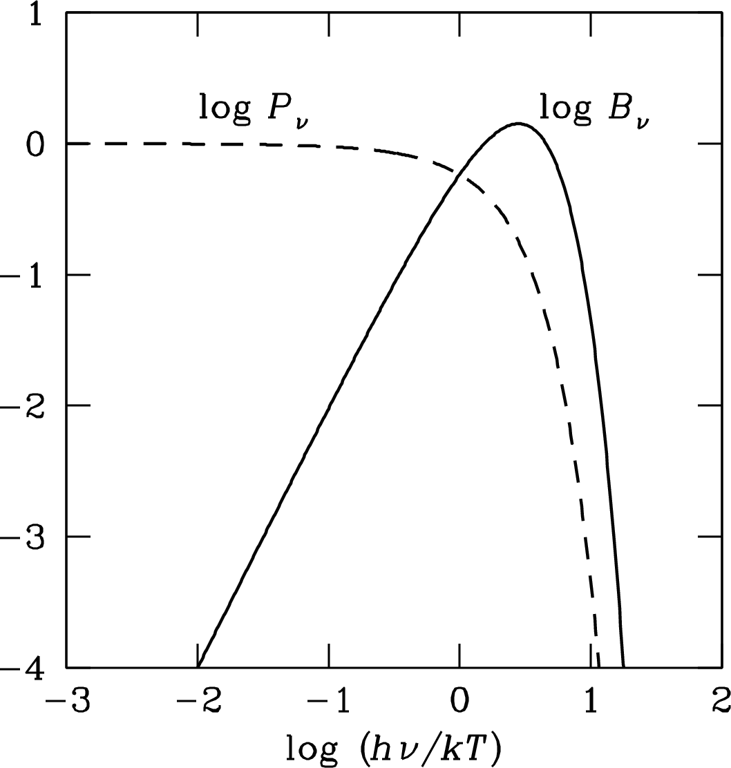
Like the Rayleigh–Jeans approximation, the Nyquist approximation implies an “ultraviolet catastrophe” that can be cured by Planck’s quantization rule. If the electrical energy in each mode is restricted to an integer multiple of , the Nyquist formula becomes
| (2.118) |
where the quantity in square brackets equals the quantization correction for blackbody radiation (Equation 2.85). The exact Nyquist formula is usually written in the form
| (2.119) |
Figure 2.20 compares the Nyquist and Planck spectra. At low frequencies , the specific intensity of blackbody radiation in three dimensions (solid curve) is proportional to . Its one-dimensional analog, the spectral power density of noise generated by a resistor (dashed curve), is proportional to . Quantization causes the sharp exponential cutoffs of both curves at high frequencies.
2.6 Cosmic Microwave Background Radiation
The universe is filled with blackbody radiation whose temperature now is . This cosmic microwave background (CMB) was produced by the hot “big bang” marking the birth of the universe. This section reviews the expanding universe, derives the evolution of blackbody radiation during the expansion, and indicates how the CMB carries cosmological information.
2.6.1 The Expanding Universe
The expanding universe is nearly homogeneous and isotropic on all scales much larger than clusters of galaxies. Consequently the recession velocity of a nearby galaxy at rest in its local environment is proportional to its (independently measured) distance . The constant of proportionality is called the Hubble parameter
| (2.120) |
is everywhere the same at any particular time after the big bang, but it changes with time. The present value of the Hubble parameter is called the Hubble constant , and its measured value is [83]
| (2.121) |
Substituting shows that the dimension of is inverse time and the Hubble constant can be written as . The Hubble time defined by
| (2.122) |
would be the present age of the universe had it started as a point and expanded at a constant rate thereafter. (The useful approximation used in Equation 2.122 is easy to remember and accurate to 0.2%.)
The radius of the observable universe is roughly the Hubble distance at which the Hubble parameter indicates a recession velocity equal to the speed of light:
| (2.123) |
It is currently .
Although general relativity is needed to describe the universe as a whole, the homogeneity of the universe means that many of its global properties can be derived by extrapolating Newtonian results obtained from regions of size . For example, the critical density is defined as the density at which the kinetic energy of expansion equals the gravitational energy decelerating the expansion. Consider a spherical region of radius centered on an observer and a unit test mass on its surface, which is receding with radial velocity . If the average density inside the sphere is , the sum of the kinetic and gravitational potential energies per unit mass will be zero:
| (2.124) | |||
| (2.125) |
so the critical density today is
| (2.126) |
for . Ordinary baryonic matter consists by mass primarily of protons and neutrons, whose masses are , so a mean number density of protons and neutrons would be needed to supply the critical density. However, in a matter-dominated universe, mutual gravitational attraction decelerates the expansion. The expansion age of a low-density () universe is nearly , but a critical-density matter-dominated universe should be only old, which is less than the ages of the oldest known stars. Dark energy actually dominates the mass-energy of the universe today, and it has the peculiar property that it accelerates the expansion enough that the actual age of the universe is closer to , eliminating the problem of stars older than the universe.
2.6.2 Blackbody Radiation in the Expanding Universe
How does the blackbody CMB evolve as the universe expands with time since the big bang? The universe is spatially homogeneous and isotropic on large scales, so the properties of the CMB can be calculated by considering what happens to blackbody radiation in a small imaginary cube whose side length slowly grows along with the universe. Here “small” only means much smaller than so that relativistic effects can be ignored; the side length might be the distance between two galaxies that are currently separated by . Although the imaginary cube has no walls, CMB radiation escaping from the cube is balanced by CMB radiation entering the cube from similar adjacent cubes. Consequently the energy density and spectrum of CMB radiation within the cube is exactly the same as that in a cubical cavity having mirrored walls and undergoing a slow adiabatic (meaning, there is no heat transfer to or from the cube) expansion. The radiation remains in equilibrium during the slow expansion, so it is always blackbody radiation.
The expansion of both the universe and the imaginary cube can be described by a single dimensionless expansion scale factor , where today. The photon number density in the cube falls as because the total number of photons in the expanding cube doesn’t change as grows. The photon number density of blackbody radiation is proportional to (Equation 2.100), so the temperature of the CMB declines as , where . Also, the mean energy per photon of blackbody radiation is proportional to . Thus the wavelength of any individual photon is proportional to , even if the photon is from a source which does not have a blackbody spectrum.
Astronomers frequently use the term redshift defined by
| (2.127) |
where and are the wavelength and frequency emitted by a source at redshift , and and are the observed wavelength and frequency at . The redshift and expansion factor are related by
| (2.128) |
Thus the CMB temperature at redshift is
| (2.129) |
The CMB radiation is ubiquitous, so interstellar matter (e.g., interstellar dust or gas) is heated by the CMB to at least the temperature given by Equation 2.129. The interstellar dust temperature in nearby galaxies like our own is , which is well above but comparable with the CMB temperature felt by galaxies at . The CMB will influence the spectral line and continuum emission visible from high-redshift galaxies.
Prior to the time corresponding to the redshift , the CMB temperature was and the radiation ionized enough of the hydrogen atoms filling the universe to keep the universe opaque. This “wall” beyond which photons cannot escape is called the surface of last scattering, and it defines the limit of the visible universe. During the recombination era when the age of the universe was only , almost all of the free protons and electrons combined to form neutral hydrogen atoms and the universe became transparent to the CMB. (The term recombination is misleading because the protons and electrons were combining for the first time.) The CMB photons received today were last scattered at that time and have been traveling in straight lines ever since, so an image of the CMB (Figure 8.16) made now () shows its temperature distribution as it was when .
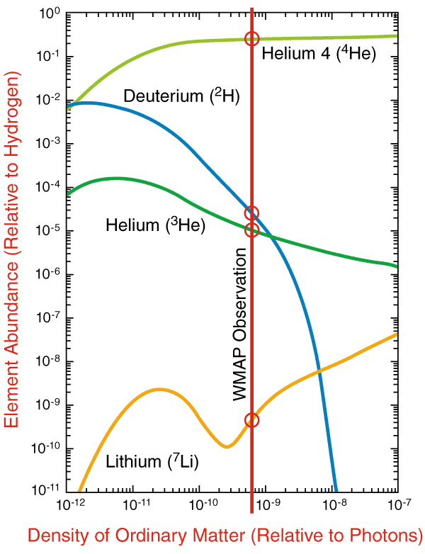
2.6.3 Prediction and Discovery of the CMB
Well before the CMB was observed, George Gamow and his students calculated the relative hydrogen and helium abundances (Figure 2.21) produced by nucleosynthesis a few minutes after a hot big bang, when the temperature of the CMB was K [2]. The abundance of deuterium in particular depends sensitively on the relative number densities of baryons (primarily protons plus neutrons by mass) and of photons . The ratio has remained constant since that time because both and and are proportional to . Equation 2.100 gives the photon number density of the CMB; it is . If , then the baryon number density is , which is only about 5% of the density needed to close the universe (Equation 2.126). Alpher and Herman [3] presented the first estimate for the present temperature of the CMB based on the chemical composition of the universe. They also showed that only light elements can be formed by big-bang nucleosynthesis because the free neutrons needed to assemble heavier elements decay with a half life of about 10 minutes. Stars produce the heavier elements.
Although is a very strong signal by radio-astronomy standards, the CMB is hard to distinguish from other noise sources in receivers and radio telescopes because it is very nearly isotropic. Unlike emission from a compact radio source, the CMB cannot be isolated by a differential measurement comparing two adjacent patches of sky. It was accidentally discovered in 1964 by Arno Penzias and Robert Wilson [81], who reported painstaking measurements indicating an isotropic “excess antenna temperature” coming from the Bell Labs horn antenna at 4080 MHz. Subsequent measurements, especially by the COBE11 1 http://lambda.gsfc.nasa.gov/product/cobe/. (COsmic Background Explorer) satellite, have demonstrated that this “excess noise” matches a blackbody spectrum within 50 parts per million well into the far infrared.
2.6.4 Dipole Anisotropy
After contamination by foreground sources near the Galactic plane has been removed, the largest observed anisotropy in the CMB is the dipole anisotropy with amplitude
| (2.130) |
where is the angle from the direction (Galactic latitude , Galactic longitude ) of the Earth’s motion relative to the universe as a whole. The speed of the Earth is much smaller than the speed of light, so the nonrelativistic Doppler equation can be used to estimate the redshift induced by the Earth’s motion:
| (2.131) |
or . This speed is consistent with the vector sum of independently measured motions of the Earth around the Sun, the Sun around the Galactic center, and the peculiar motion of our Galaxy in the local universe.
2.6.5 Intrinsic Anisotropy
The age of the universe at recombination can be calculated because the physics of the homogeneous and isotropic early universe was so simple. During that time, small inhomogeneities in the density of dark matter were amplified by gravity. Baryons started falling into the gravitational potential wells, and the CMB was coupled to this flow by Thomson scattering (Equation 5.33) off the numerous free electrons present prior to . Radiation pressure resisted this infall, setting up baryon acoustic oscillations analogous to sound vibrations in air, but with a “sound” speed . The strongest oscillations in the CMB brightness had wavelengths equal to the diameter of the sound horizon at the time of recombination:
| (2.132) |
which was about . After recombination, the photons decoupled and this “standard ruler” grew by a factor ( to its present size of . Figure 8.16 shows these CMB brightness fluctuations, projected onto a sphere [106]. The angular power spectrum of CMB fluctuations (Figure 1.16) observed by the Wilkinson Microwave Anisotropy Probe (WMAP) and by the Planck Mission reveal that the angular size of this ruler is , so the comoving distance to the surface of last scattering is . The radius of the observable universe (including gravitational radiation and neutrinos from redshifts ) is only about 2% larger. If we live in a flat CDM universe ( Cold Dark Matter universe, where stands for the cosmological constant associated with dark energy), its present age is .
The intrinsic rms of the CMB over the whole sky is , which is only about of the average . This leads to the horizon problem: Why should the CMB temperature be the same at points separated by more than , which were never in causal contact by the time of recombination? The simple big-bang model also has a flatness problem. The universe is nearly “flat” today so its density is close to the critical density, and it must have been much closer to the critical density when it was much smaller (e.g., during the nucleosynthesis era when ). What “fine tuned” the density of the universe?
The preferred solution for both problems is that the early universe underwent a brief period () of inflation during which the scale factor grew exponentially by a factor . The observable universe is only an infinitesimal and causal part of the whole universe, nearly all of which is outside our horizon. The vacuum energy associated with inflation ensures that the total density contributed by both matter and energy approaches the critical density.
2.7 Radiation from an Accelerated Charge
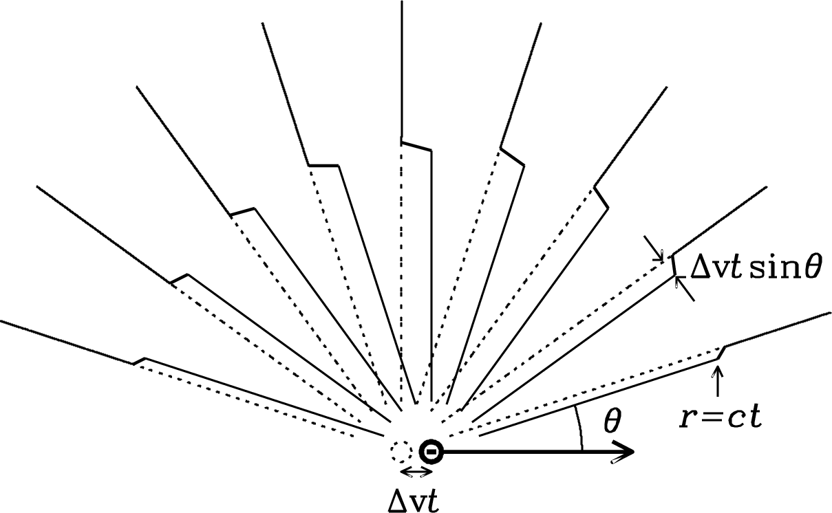
Maxwell’s equations imply that all classical electromagnetic radiation is generated by accelerating electrical charges. It is possible to derive the intensity and angular distribution of the radiation from a point charge (a charged particle) subject to an arbitrary but small acceleration via Maxwell’s equations, but the complicated math obscures the physical interpretation that remains clear in J. J. Thomson’s illuminating derivation (see [69]).
If a particle with electrical charge is at rest or moving with a constant velocity, its electric field lines are purely radial: . Suppose a charged particle initially at rest is accelerated to a small velocity in a short time . This disturbs the lines of force, and the disturbance travels outward at the speed of light . Figure 2.22 shows that at time after the acceleration, the disturbance will have propagated to and the perpendicular component of the electric field will have magnitude
| (2.133) |
where is the angle between the acceleration vector and the line of sight connecting the charge to the observer. The web applet https://phet.colorado.edu/en/simulation/radiating-charge provides a very clear and interactive demonstration of this effect.
Coulomb’s law for the radial component of the electric field (electric force per unit charge) a distance from a stationary charge is
| (2.134) |
in Gaussian CGS units. Substituting for in Equation 2.133 and using Coulomb’s law to eliminate gives
| (2.135) |
and
| (2.136) |
where
| (2.137) |
Equation 2.136 is valid for any small acceleration, not just a sinusoidal acceleration at a single frequency. The transverse field at mimics the acceleration at . Thus a sinusoidal acceleration would result in a sinusoidal variation of with the same frequency.
Notice that (Equation 2.136) falls more slowly with distance than (Equation 2.134). Far from the charged particle, only will contribute significantly to the observed electric field. From a distant observer’s point of view, only the “visible” component of acceleration perpendicular to the line of sight () contributes to the radiated electric field; the “invisible” component of acceleration parallel to the line of sight () does not appear to radiate—what you see is what you get. Likewise, the radiated electric field is linearly polarized in the direction parallel to the component of acceleration perpendicular to the line of sight.
How much power is radiated in each direction? The Poynting flux, or power per unit area (e.g., erg s cm), is
| (2.138) |
In CGS units so
| (2.139) |
Inserting Equation 2.136 into Equation 2.139 gives
| (2.140) |
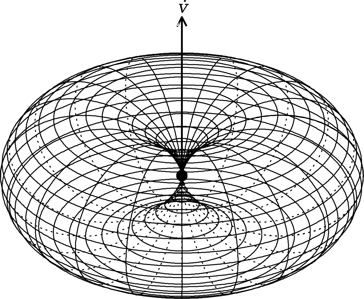
at large distances . The accelerated charge radiates with a dipolar power pattern shaped like a doughnut whose axis is parallel to the acceleration (Figure 2.23).
The total power emitted is the integral of over the spherical surface of radius :
| (2.141) | ||||
| (2.142) |
The integral , so the total power emitted by the accelerated charged particle is
| (2.143) |
This result is called Larmor’s equation. It implies that any charged particle radiates when accelerated and that the total radiated power is proportional to the square of the acceleration. The largest astrophysical accelerations are usually produced by electromagnetic forces, so the acceleration is proportional to the charge/mass ratio of the particle. In celestial sources, radiation from electrons is typically ( times stronger than radiation from protons.
Larmor’s extremely useful equation will be the basis for our derivations of radiation from a short dipole antenna as well as for free–free and synchrotron emission from astrophysical sources. Beware that Larmor’s formula is nonrelativistic; it is valid only in frames moving at velocities with respect to the radiating particle. To treat particles moving at nearly the speed of light in the observer’s frame, we must first use Larmor’s equation to calculate the radiation in the particle’s rest frame and then transform the result to the observer’s frame in a relativistically correct way. Also, Larmor’s formula does not incorporate the constraints of quantum mechanics, so it should be applied only with great caution to microscopic systems such as atoms. For example, Larmor’s equation incorrectly predicts that the electron orbiting in the lowest energy level of a hydrogen atom will quickly radiate away all of its kinetic energy and fall into the nucleus. On the other hand, it correctly predicts the radio power emitted by an electron orbiting in a very high energy level of a hydrogen atom.
2.8 Dust Emission at Radio Wavelengths
All small solid particles in space are called dust grains by astronomers. Interstellar dust was first recognized because it scatters or absorbs ultraviolet, visible, and near-infrared photons from stars. Extinction is defined as the total dimming of the light coming directly from a point source caused by both photon scattering and photon absorption, and it is usually expressed in units of . The amount of extinction is inversely proportional to wavelength for , indicating that the grains responsible have sizes . Interstellar dust grains are much smaller than common terrestrial dust particles visible to the naked eye, and they are much smaller than the wavelengths (frequencies ) accessible to ground-based radio astronomy (Figure 1.3).
Dust scattering occurs because the oscillating electric field of incident radiation forces electrons within dust grains to oscillate and hence reradiate at the same frequency in all directions, as shown in Section 2.7. In the radio limit these radiators are very inefficient, so their scattering cross section is proportional to (Rayleigh’s law). Rayleigh’s law applies to all small grains, regardless of composition. Scattering in the limit is called Rayleigh scattering, and Rayleigh scattering of sunlight by air molecules is why the sky is so blue and the setting Sun is so red. Although photon scattering by dust in front of a star makes the star appear both dimmer and redder in color, scattering by dust within an extended object such as an external galaxy affects neither its total brightness nor its color. Only the absorption component of its internal dust extinction can redden or dim an external galaxy.
Some of the incident photons are absorbed, and their energy heats the dust grains. The energy carried by a single ultraviolet photon can significantly raise the temperature of a very small () dust grain, so the smallest grains are not in thermodynamic equilibrium with the local interstellar radiation field. Larger interstellar dust grains have enough heat capacity to come into equilibrium at well-defined temperatures such that the power absorbed is balanced by power reemitted primarily at far-infrared (FIR) wavelengths . The nearly equal UV/optical and FIR peaks in the cosmic background (Figure 1.4) imply that about half of all UV/optical starlight escapes and half is absorbed within its parent galaxy. This result is an average over all galaxies, but individual galaxies can range from nearly transparent (e.g., elliptical galaxies with little interstellar dust) to nearly opaque (e.g., the compact ultraluminous starburst galaxy Arp 220).
The dust absorption cross section varies as when , so at radio wavelengths (1) dust absorption () contributes much more than dust scattering () to the total extinction, and (2) all galaxies are nearly transparent. Thus radio (and far-infrared ) observations can see into dusty starburst galaxies, and the radio/FIR luminosity is nearly proportional to the recent rate of star formation, unaffected by dust obscuration.
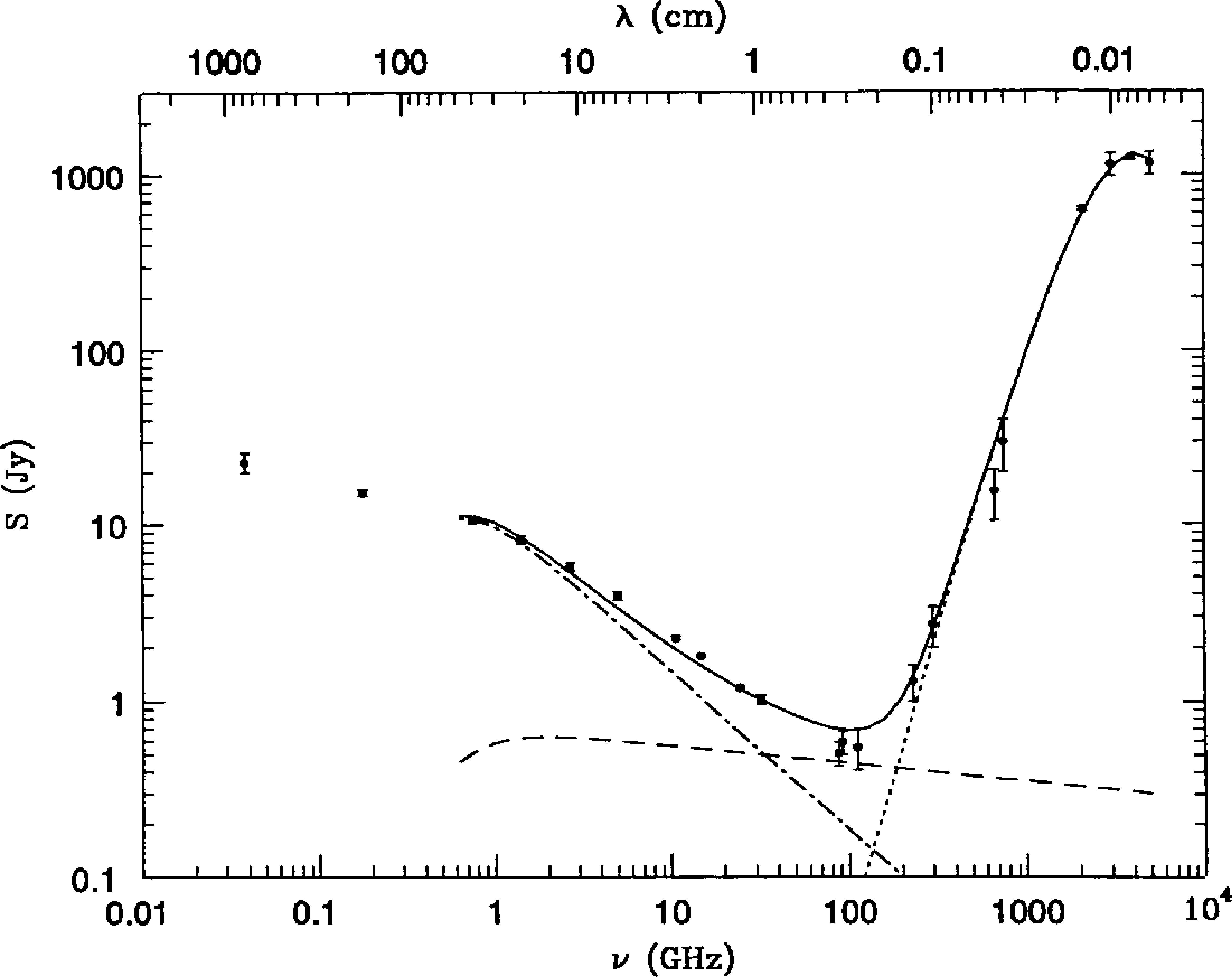
Obeying Kirchhoff’s law for opaque bodies (Equation 2.47), small dust grains are also inefficient emitters. Their absorption and emission coefficients both scale with frequency as , where and in the Rayleigh limit. Thus dusty radio sources do not have Rayleigh–Jeans radio spectra ; they have relatively “blue” spectra rising as . The dotted curve in Figure 2.24 showing dust emission from the galaxy M82 indicates to for .
A striking consequence of such a steeply rising spectrum is that the flux density of a galaxy observed through the () atmospheric window (Figure 1.3) is nearly independent of its redshift in the range . The strongest submm galaxies tend to be the most luminous, and radio surveys at wavelengths near are effective at tracing the rate of star formation over the entire redshift range during which most stars formed [10].
Astronomical dust is also present in protoplanetary disks. These “dust” particles are much larger than interstellar dust grains, so they can be strong radio emitters with nearly blackbody spectra at . The spectacular ALMA (Figure 8.5) image of the dust disk surrounding the young star HL Tau (Figure 8.9) has sufficient angular resolution () to show dark rings carved out by young planets [1].