Chapter 5 Synchrotron Radiation
5.1 Magnetobremsstrahlung
Any accelerated charged particle emits electromagnetic radiation with power specified by Larmor’s formula (Equation 2.143). In astrophysical situations, electromagnetic forces produce the strongest accelerations of charged particles. Acceleration by an electric field accounts for free–free radiation. Acceleration by a magnetic field produces magnetobremsstrahlung, the German word for “magnetic braking radiation.” The lightest charged particles (electrons, and positrons if any are present) are accelerated more than relatively massive protons and heavier ions, so electrons (and possibly positrons) account for virtually all of the radiation observed. The character of magnetobremsstrahlung depends on the speeds of the electrons, so these somewhat different types of radiation are given specific names. Gyro radiation comes from electrons whose velocities are much smaller than the speed of light: . Mildly relativistic electrons whose kinetic energies are comparable with their rest mass emit cyclotron radiation, and ultrarelativistic electrons (kinetic energies ) produce synchrotron radiation.
Synchrotron radiation is ubiquitous in astronomy. It accounts for most of the radio emission from active galactic nuclei (AGNs) thought to be powered by supermassive black holes in galaxies and quasars, and it dominates the radio continuum emission from star-forming galaxies like our own at frequencies below GHz. The magnetosphere of Jupiter is a synchrotron radio source. The optical emission from the Crab Nebula supernova remnant, the optical jet of the radio galaxy M87, and the optical through X-ray emission from many quasars is synchrotron radiation.
The relativistic electrons in nearly all synchrotron sources have power-law energy distributions, so they are not in local thermodynamic equilibrium (LTE). Consequently, synchrotron sources are often called “nonthermal” sources. However, a synchrotron source with a relativistic Maxwellian electron-energy distribution would be a thermal source, so “synchrotron” and “nonthermal” are not completely synonymous.
Even though synchrotron radiation is quite different from free–free emission, notice how many themes from the derivation of free–free source spectra are repeated for synchrotron sources—Larmor’s equation is used to derive the total power and spectrum of radiation by a single electron, the spectrum of an optically thin source is obtained as the superposition of the spectra of individual electrons, the electron energy distribution is broad enough that the spectrum of an individual electron can be approximated by a delta function, Kirchhoff’s law yields the absorption coefficient in terms of the emission coefficient (even though the synchrotron source is not in LTE!), and the simple “cylindrical cow” geometry is used to yield the spectrum of a source that is optically thick at low frequencies.
5.1.1 Gyro Radiation
Larmor’s equation is valid only for gyro radiation from a particle with charge moving with a small velocity . The magnetic force exerted on the particle by a magnetic field is
| (5.1) |
The magnetic force is perpendicular to the particle velocity, so . Consequently the magnetic force does no work on the particle, does not change the particle’s kinetic energy , and does not change the component of velocity parallel to the magnetic field. Because both and are constant, the magnitude of the velocity component perpendicular to the magnetic field must also be constant. In a uniform magnetic field, the particle moves along the magnetic field line on a helical path with constant linear and angular speeds. In the inertial frame moving with velocity , the particle orbits in a circle of radius perpendicular to the magnetic field with the angular velocity needed to balance the centripetal and magnetic forces:
| (5.2) |
the orbital angular frequency is
| (5.3) |
Equation 5.3 implies that the orbital frequency is independent of the particle speed so long as . The angular gyro frequency is defined by
| (5.4) |
This definition holds for any particle speed, so the gyro frequency equals the actual orbital frequency if and only if .
The angular gyro frequency (rad s) of an electron is
| (5.5) | ||||
| (5.6) |
In terms of the electron gyro frequency in MHz is
| (5.7) |
The typical interstellar magnetic field strength in a normal spiral galaxy like ours is G, so the electron gyro frequency is only . The associated gyro radiation cannot propagate through the ISM because its frequency is less than the plasma frequency (Equation 6.40).
Gyro radiation from nonrelativistic electrons is observable in very strong magnetic fields such as the gauss magnetic field of a neutron star. For example, the binary X-ray source Hercules X-1 exhibits an X-ray absorption line at photon energy keV (Figure 5.1).
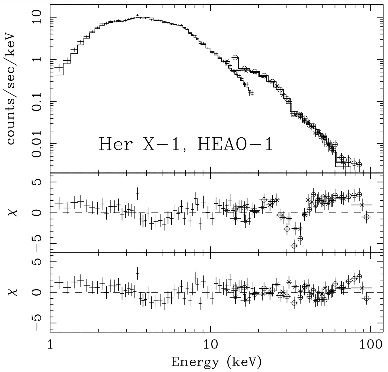
This spectral feature is thought to be a gyro-resonance absorption, in which case the frequency of this absorption line directly measures the magnetic field strength near the Her X-1 neutron star. The observed photon energy corresponds to the frequency
| (5.8) |
Equating this frequency to the gyro frequency yields the magnetic field:
| (5.9) | ||||
| (5.10) | ||||
| (5.11) |
5.2 Synchrotron Power
Cosmic rays are celestial particles (e.g., electrons, protons, and heavier nuclei) with extremely high energies. Cosmic-ray electrons in the interstellar magnetic field emit the synchrotron radiation that accounts for most of the continuum emission from our Galaxy at frequencies below about 30 GHz. Larmor’s formula can be used to calculate the synchrotron power and synchrotron spectrum of a single electron in the inertial frame in which the electron is instantaneously at rest, but the Lorentz transform of special relativity is needed to transform these results to the frame of an observer at rest in the Galaxy.
5.2.1 Lorentz Transforms
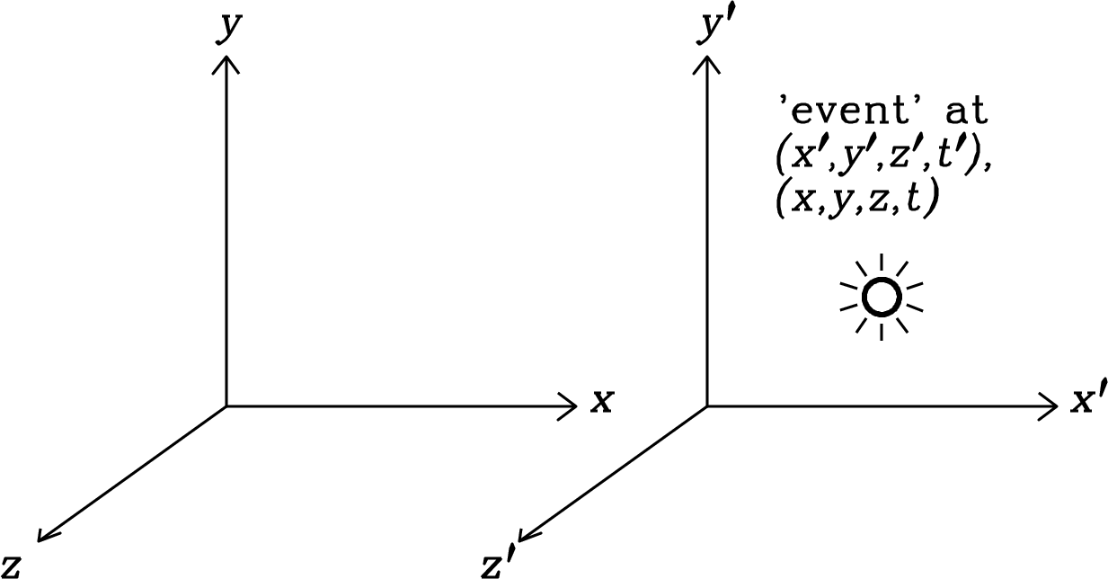
For any pointlike event, the Lorentz transform (see Appendix C for a derivation) relates the coordinates in the unprimed inertial frame and the coordinates in the primed frame moving with velocity in the -direction (Figure 5.2). They are
| (5.12) |
| (5.13) |
where
| (5.14) |
and
| (5.15) |
is called the Lorentz factor. The Lorentz transform is linear, so even for finite coordinate differences and between two events, the differential form of the Lorentz transform is
| (5.16) |
| (5.17) |
5.2.2 Relativistic Masses
The rest mass of an electron can be converted to an energy by Einstein’s famous mass–energy equation
| (5.18) |
The energy corresponding to the electron’s rest mass is
| (5.19) | ||||
| (5.20) |
Cosmic-ray electrons having masses (Equation C.28) and total energies are called ultrarelativistic.
Ultrarelativistic electrons still move on spiral paths along magnetic field lines, but the angular frequencies of their orbits are lower because their inertial masses are multiplied by (Appendix C):
| (5.21) |
The orbital frequency of a cosmic-ray electron with in a G interstellar magnetic field is only
| (5.22) |
Because whenever , the orbital radius of an ultrarelativistic electron is nearly independent of and can be quite large:
| (5.23) |
Equation 5.21 is not promising for the production of observable synchrotron radiation: the high observed masses of relativistic electrons reduce their orbital frequencies and accelerations to extremely low values. However, two compensating relativistic effects can explain the strong synchrotron radiation observed at radio frequencies: (1) the total radiated power in the observer’s frame is proportional to and (2) relativistic beaming turns the low-frequency sinusoidal radiation in the electron frame into a series of extremely sharp pulses containing power at much higher frequencies in the observer’s frame. These relativistic corrections are derived in Sections 5.2.3 and 5.3.1.
5.2.3 Synchrotron Power Radiated by a Single Electron
Let primed coordinates describe the inertial frame in which the electron is (temporarily) nearly at rest. Larmor’s equation (Equation 2.143) gives the radiated power in the electron rest frame as
| (5.24) |
because (electric charge is a relativistic invariant) follows directly from Maxwell’s relativistically correct equations.
The magnetic acceleration of the electron in the frame of an observer at rest in the Galaxy can be derived by applying the chain rule for derivatives to the differential Lorentz coordinate transform (Equations 5.16 and 5.17).
| (5.25) |
Similarly, so
| (5.26) |
Thus
| (5.27) |
The next step is to transform from the radiated power in the electron frame to , the power measured by an observer at rest in the Galaxy, by applying the chain rule to the mass–energy Equation 5.18:
| (5.28) |
that is, the power is a relativistic invariant. Consequently,
| (5.29) |
To calculate , combine force balance in a circular orbit
| (5.30) |
with Equation 5.21 for to get
| (5.31) |
where the constant angle between the electron velocity and the magnetic field is called the pitch angle.
Inserting from Equation 5.31 into Equation 5.29 gives the power radiated by a single electron moving with pitch angle :
| (5.32) |
This power is usually written in terms of the Thomson cross section of an electron, . The Thomson cross section is the classical radiation-scattering cross section of a charged particle. If a plane wave of electromagnetic radiation passes a free charged particle initially at rest, the electric field of that radiation will accelerate the particle, which in turn will radiate power in all directions according to Larmor’s equation. This process is called scattering rather than absorption because the total power in electromagnetic radiation is unchanged—all of the power extracted from the incident plane wave is reradiated at the same frequency but in other directions. It is a straightforward exercise to show that the geometric area that would intercept this amount of incident power from the plane wave is
| (5.33) |
Numerically,
| (5.34) |
The reason for using the Thomson cross section will become clear in the discussion of inverse-Compton scattering of radiation by the same cosmic rays that are producing synchrotron radiation (Section 5.5.1).
It is also conventional to eliminate the in Equation 5.32 in favor of the magnetic energy density
| (5.35) |
Then
| (5.36) |
simplifies to
| (5.37) |
The synchrotron power radiated by a single electron depends only on physical constants, the square of the electron kinetic energy (via ), the magnetic energy density , and the pitch angle .
The relativistic electrons in radio sources can have lifetimes of thousands to millions of years before losing their ultrarelativistic energies via synchrotron radiation or other processes. During their lifetimes they are scattered repeatedly by magnetic-field fluctuations and charged particles in their environment, and the distribution of their pitch angles gradually becomes random and isotropic. The average synchrotron power per electron in an ensemble of electrons having the same Lorentz factor and isotropically distributed pitch angles is
| (5.38) |
where is the average over all pitch angles:
| (5.39) | ||||
| (5.40) | ||||
| (5.41) |
Thus the average synchrotron power per relativistic electron in a source with an isotropic pitch-angle distribution is
| (5.42) |
For all , the factor can be ignored. Relativistic effects multiply the average radiated power by a factor compared with the nonrelativistic () Larmor equation.
5.3 Synchrotron Spectra
5.3.1 The Synchrotron Spectrum of a Single Electron
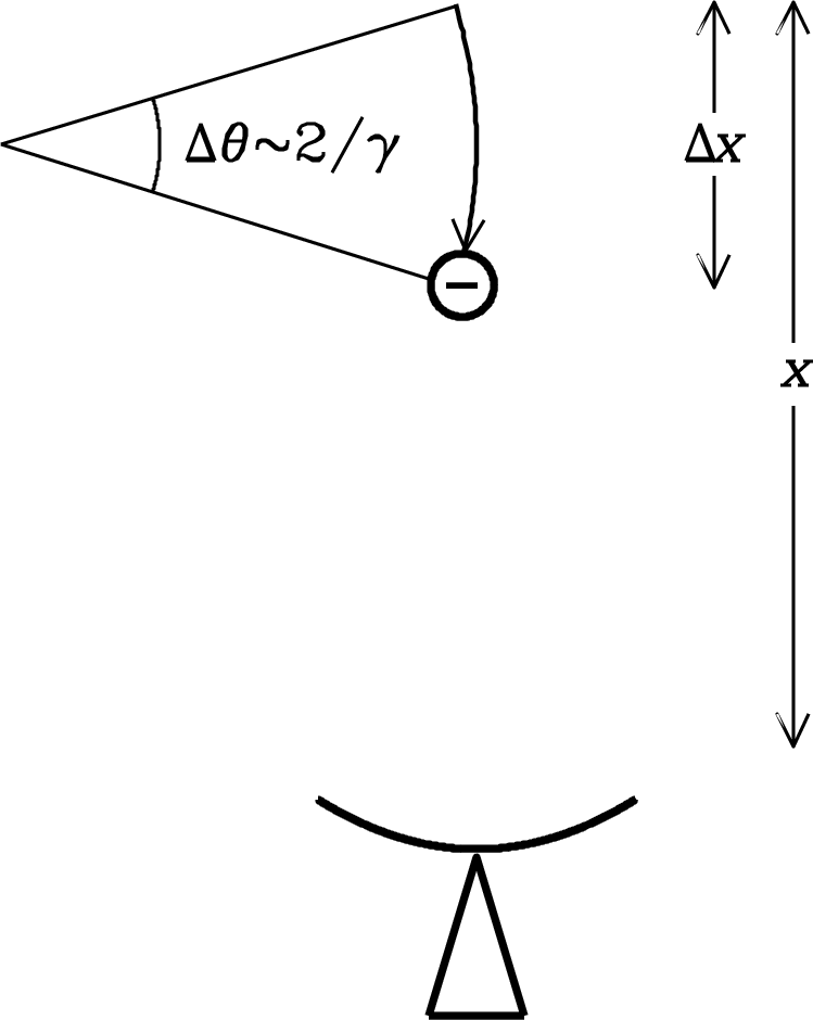
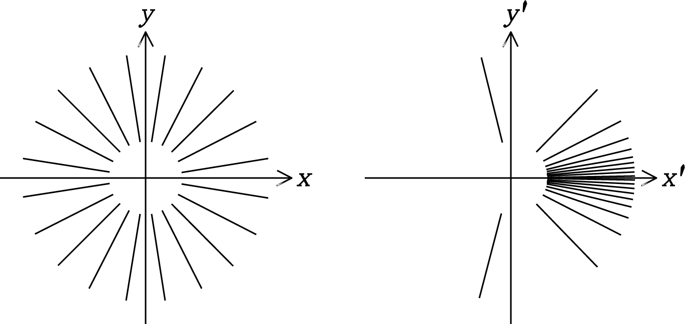
Why does synchrotron radiation appear at frequencies much higher than ? First, relativistic aberration beams the dipole pattern of Larmor radiation in the electron frame sharply along the direction of motion in the observer’s frame as approaches (Figure 5.3). Relativistic photon beaming follows directly from the relativistic velocity addition equations (Equations C.22 through C.26) that relate the photon velocity component in the unprimed frame of the observer to the photon velocity component in the primed frame and the velocity of the primed frame in which the electron is instantaneously at rest:
| (5.43) | ||||
| (5.44) |
| (5.45) |
In the -direction,
| (5.46) |
| (5.47) |
Consider the synchrotron photons emitted with speed at an angle from the -axis. Let and be the projections of the photon speed onto the - and -axes. Then
| (5.48) |
In the observer’s frame the same photons have
| (5.49) |
Inserting the velocity Equations 5.45 and 5.47 into the angle Equations 5.48 and 5.49 yields relations connecting and :
| (5.50) |
and
| (5.51) |
In the frame moving with the electron, the Larmor equation implies a power pattern proportional to with nulls at . In the observer’s frame, these nulls are offset by much smaller angles
| (5.52) |
An observer at rest sees the radiation confined to a very narrow beam of width between nulls, as shown in Figure 5.3. For example, a 10 GeV electron has so arcsec! Although the electron is emitting continuously, the observer sees a short pulse of radiation only from the tiny fraction
| (5.53) |
of the electron orbit where the electron is moving almost directly toward the observer.

The duration of the observed pulse is even shorter than the time the electron needs to cover of its orbit because the electron is moving almost directly toward the observer with a speed approaching (Figure 5.4) when it is observable. As it travels toward the observer, the electron nearly keeps up with the radiation that it emits:
| (5.54) | ||||
| (5.55) |
The first term in this equation represents the time taken by the electron to cover the distance , the second is the light travel time from the electron position at the end of the pulse seen by the observer, and the third is the light travel time from the electron position at the beginning of the pulse seen by the observer. Note that the observed pulse duration
| (5.56) |
is much less than the time the electron needs to move a distance because, in the observer’s frame, the electron nearly keeps up with its own radiation. In the limit ,
| (5.57) |
so
| (5.58) |
Recall that (Figure 5.4) so
| (5.59) |
is the full observed duration of the pulse. Allowing for the motion of the electron parallel to the magnetic field replaces the total magnetic field by its perpendicular component , yielding
| (5.60) |
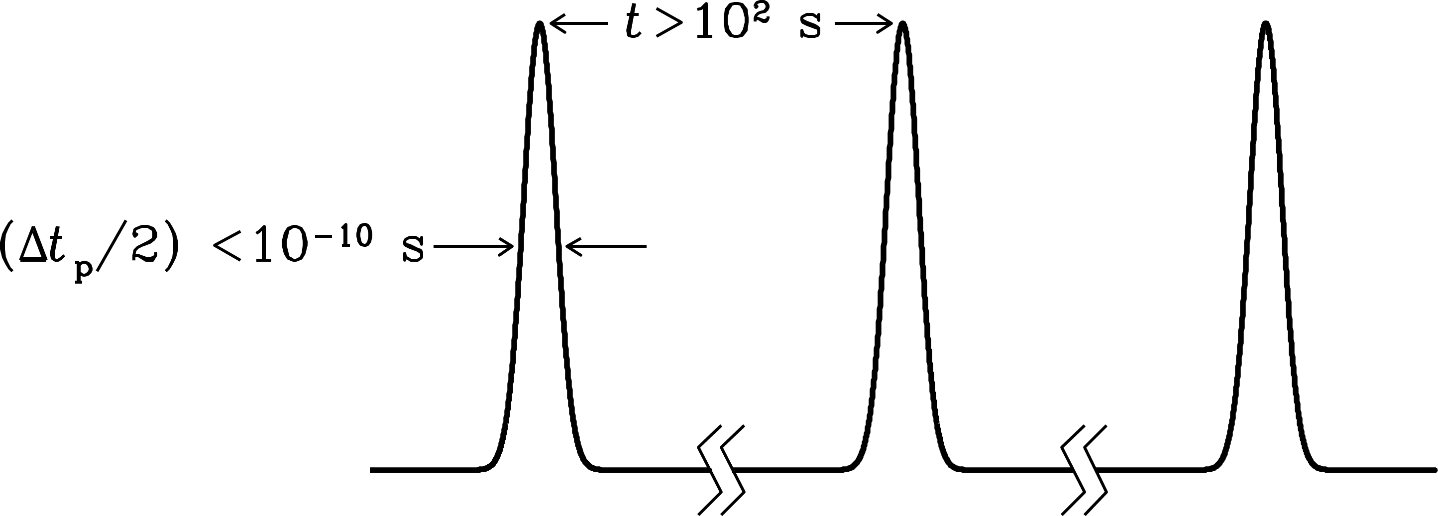
where is the pitch angle of the electron. Thus a plot of the power received as a function of time is very spiky. If and G, the half width of each pulse is s and the spacing between pulses is s (Figure 5.5).
The observed synchrotron power spectrum is the Fourier transform of this time series of pulses. The pulse train is the convolution of the individual pulse profile with the shah function (see Figure A.1 or Bracewell [15], a valuable reference book):
| (5.61) |
where each delta function is an infinitesimally narrow spike at integer and whose integral is unity. The convolution theorem (Equation A.15) states that the Fourier transform of the pulse train is the product of the Fourier transform of one pulse and the Fourier transform of the shah function.
The Fourier transform of the shah function is also the shah function (Figure A.1), so the similarity theorem (Equation A.11) implies that the Fourier transform of
| (5.62) |
in the time domain is proportional to
| (5.63) |
which is a nearly continuous series of spikes in the frequency domain. Adjacent spikes are separated in frequency by only
| (5.64) |
Although this is not formally a continuous spectrum, the frequency shifts caused by even tiny fluctuations in electron energy, magnetic field strength, or pitch angle cause frequency shifts much larger than , so the spectrum of synchrotron radiation is effectively continuous.
Thus the synchrotron spectrum of a single electron is fairly flat at low frequencies and tapers off at frequencies above
| (5.65) |
It isn’t necessary to know the Fourier transform of the pulse shape precisely to calculate the synchrotron spectra of celestial sources because real sources don’t contain electrons with just one energy and one pitch angle in a uniform magnetic field. The actual energy distribution of cosmic rays in a real radio source is a very broad power law, broad enough to smear out the details of the spectrum from each electron-energy range. Just for the record, the synchrotron power spectrum of a single electron is
| (5.66) |
where is a modified Bessel function and is the critical frequency whose value is
| (5.67) |
For the full mathematical derivation of Equations 5.66 and 5.67, see Pacholczyk [78], a valuable reference for details of radiation processes.
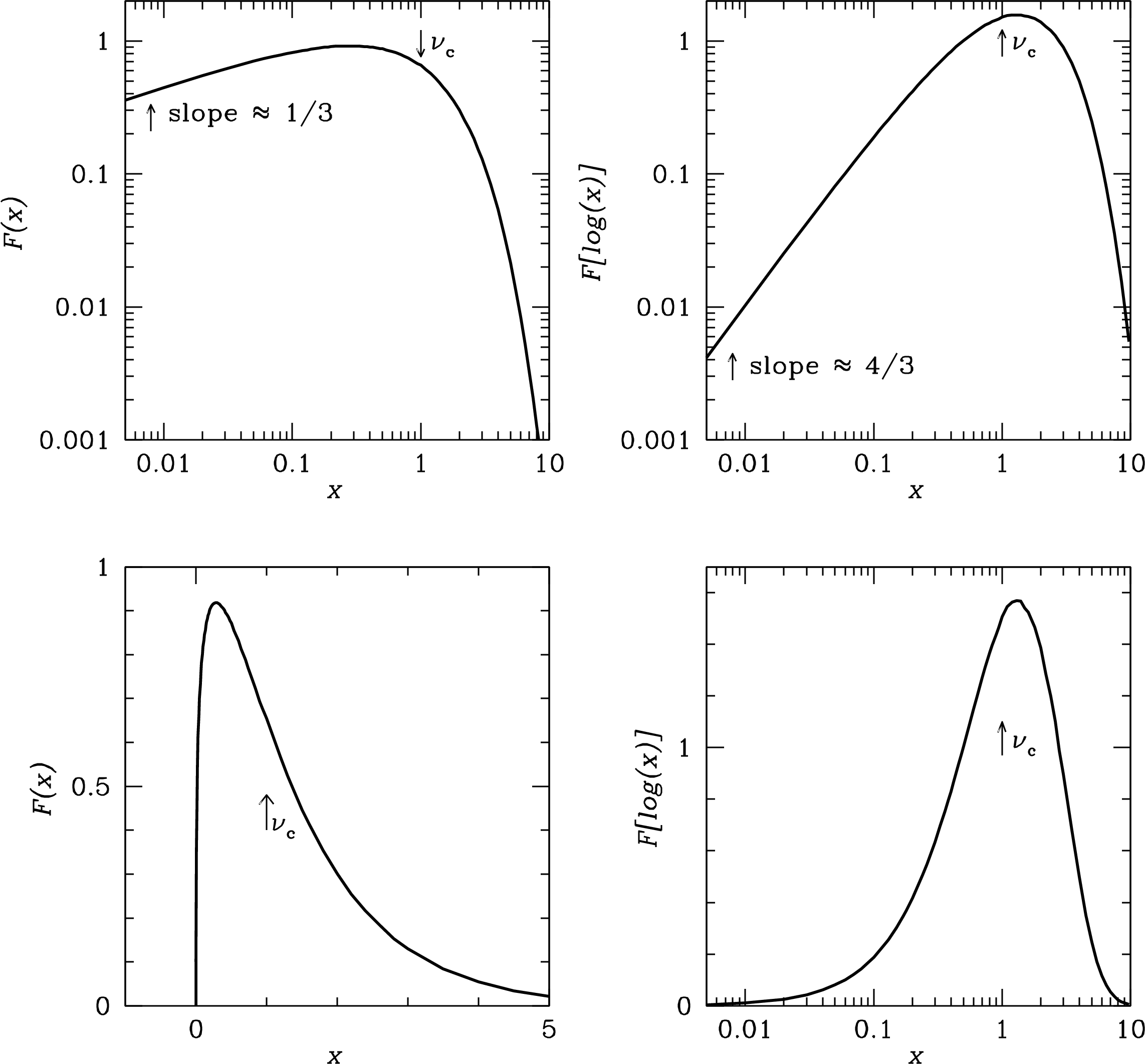
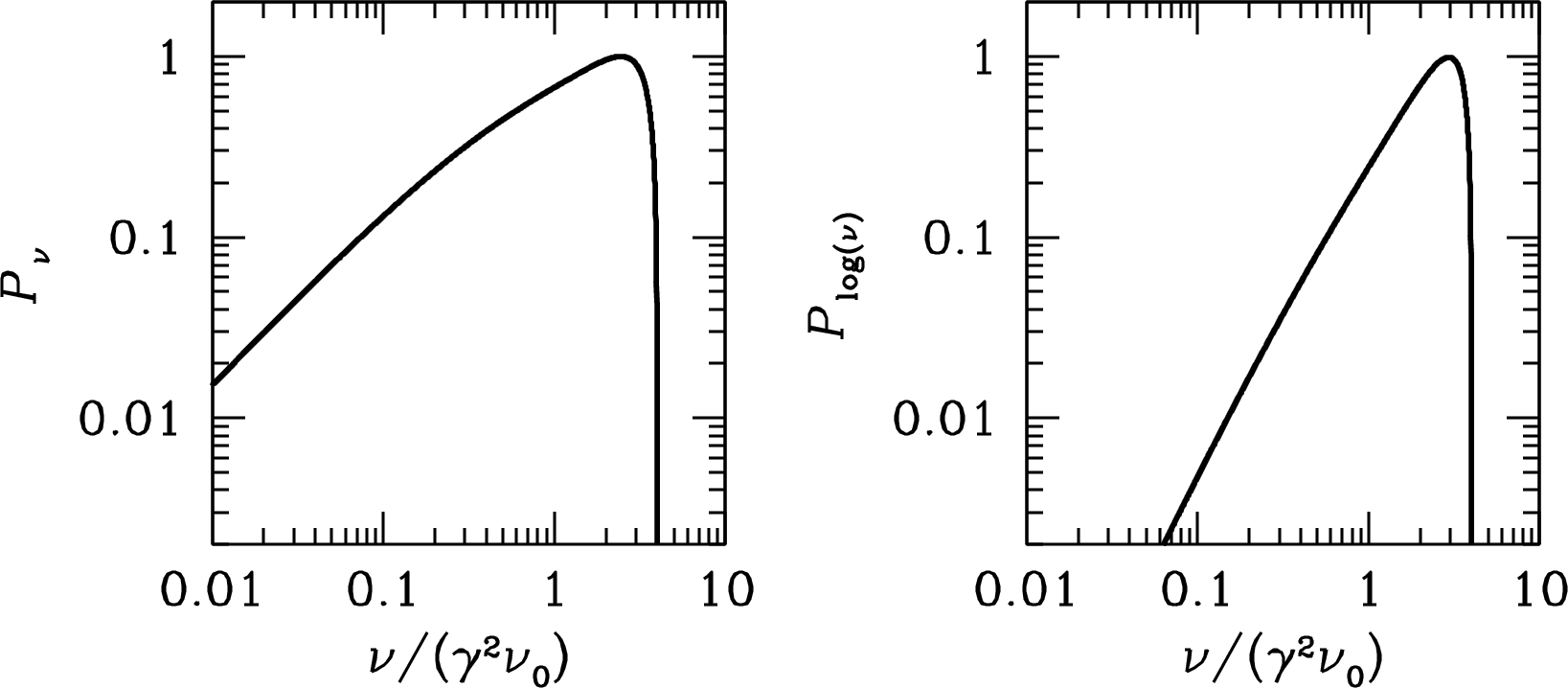
The synchrotron power spectrum of a single electron is plotted in Figure 5.6. It has a logarithmic slope
| (5.68) |
at low frequencies, a broad peak near the critical frequency , and falls off sharply at higher frequencies. One way to look at is
| (5.69) |
That is, the frequency at which each electron emits most strongly is proportional to the square of its energy multiplied by the strength of the perpendicular component of the magnetic field.
5.3.2 Synchrotron Spectra of Optically Thin Radio Sources
If a synchrotron source containing any arbitrary distribution of electron energies is optically thin (), then its spectrum is the superposition of the spectra from individual electrons and its flux density cannot rise faster than at any frequency . In other words, the (negative) spectral index (be careful not to confuse this spectral index with the electron pitch angle ) must always be greater than . Most astrophysical sources of synchrotron radiation have spectral indices near at frequencies where they are optically thin, and their high-frequency spectral indices reflect their electron energy distributions, not the spectra of individual electrons.
The energy distribution of cosmic-ray electrons in most synchrotron sources is roughly a power law:
| (5.70) |
where is the number of electrons per unit volume with energies to . The energy range around is relevant to the production of radio radiation. Because is nearly a power law over more than a decade of energy and the critical frequency is proportional to , the synchrotron spectrum will reflect this power law over a frequency range of at least . Consequently the detailed spectra of individual electrons can be ignored because they are smeared out in the source spectrum by the broad power-law energy distribution. The source spectrum can be calculated with good accuracy from the approximation that each electron radiates all of its average power (Equation 5.42)
| (5.71) |
at the single frequency
| (5.72) |
which is very close to the critical frequency (Equation 5.67). Then the emission coefficient (Equation 2.26) of synchrotron radiation by an ensemble of electrons is
| (5.73) |
where
| (5.74) |
Differentiating in Equation 5.74 gives
| (5.75) |
so
| (5.76) |
Eliminating in favor of and then using yields an expression for in terms of and only:
| (5.77) |
This simplifies to
| (5.78) |
Thus the spectrum of optically thin synchrotron radiation from a power-law distribution of electrons is also a power law, and the spectral index depends only on :
| (5.79) |
In our Galaxy and in many other synchrotron sources, near GHz, so the radio spectra imply . This value of reflects the initial power-law energy slope of cosmic rays accelerated in shocks, such as the shocks produced by supernova remnants expanding into the ambient interstellar medium, modified by loss processes that deplete the population of relativistic electrons. For example, the rate at which an electron loses energy to synchrotron radiation is proportional to , so higher-energy electrons are depleted more rapidly. The critical frequency is also proportional to , so synchrotron losses eventually steepen source spectra at higher frequencies. If relativistic electrons with initial power-law slope are continuously injected into a synchrotron source, synchrotron losses will eventually steepen that slope to at high energies and the high-frequency spectral index will steepen by . See Pacholczyk [78] for a more detailed discussion of energy losses and their spectral consequences.
5.3.3 Synchrotron Self-Absorption
The brightness temperatures of synchrotron sources cannot become arbitrarily large at low frequencies because for every emission process there is an associated absorption process. If the emitting particles are in local thermodynamic equilibrium (LTE), they have a Maxwellian energy distribution and the source is thermal. No thermal source can have a brightness temperature greater than the kinetic temperature of the emitting particles. If the energy distribution of relativistic electrons in a synchrotron source were a (relativistic) Maxwellian, the electrons would have a well-defined kinetic temperature, and synchrotron self-absorption would prevent the brightness temperature of the synchrotron radiation from exceeding the kinetic temperature of the emitting electrons. Most astrophysical synchrotron sources are nonthermal sources because the energy distribution of the relativistic electrons is a power law and there is no well-defined electron temperature. However, synchrotron self-absorption occurs for any electron energy distribution, and the low-frequency spectrum of an optically thick synchrotron source is a power law whose slope is . That result is derived below.
Electrons with energy emit most of their synchrotron power near the critical frequency
| (5.80) |
so the synchrotron emission at frequency comes primarily from electrons with Lorentz factors near
| (5.81) |
In this approximation that only those electrons having one particular energy contribute to the emission (and hence absorption) at each frequency , all other electrons could have a relativistic Maxwellian energy distribution to match without changing the resulting emission and absorption at that frequency. Consequently, a sufficiently bright synchrotron source will be optically thick, and its brightness temperature at any frequency cannot exceed the effective temperature of the electrons emitting at that frequency.
In an ultrarelativistic gas, the ratio of specific heats at constant pressure and at constant volume is , not the nonrelativistic , so the relation between electron energy and temperature is
| (5.82) |
Thus the effective temperature of relativistic electrons with energy can be defined as
| (5.83) |
even if the ensemble of electrons has a nonthermal energy distribution. Using Equation 5.81 to eliminate in favor of gives the effective temperature of those electrons producing most of the synchrotron radiation at frequency :
| (5.84) |
Numerically,
| (5.85) |
For example, the effective temperature of the relativistic electrons emitting synchrotron radiation at in a gauss gauss magnetic field is
| (5.86) |
At a sufficiently low frequency , the brightness temperature of any synchrotron source will approach the effective electron temperature of electrons emitting at that frequency and the source will become opaque. Equation 2.33 defines brightness temperature in the Rayleigh–Jeans limit:
| (5.87) |
Setting and using Equation 5.85 to eliminate in favor of and gives
| (5.88) |
Thus at low frequencies the spectrum of a synchrotron self-absorbed and spatially homogeneous source is a power law of slope :
| (5.89) |
independent of the slope of the electron-energy spectrum. The flux density of an opaque but truly thermal source (e.g., an Hii region) is proportional to ; the extra for synchrotron radiation comes from the fact that (Equation 5.85).
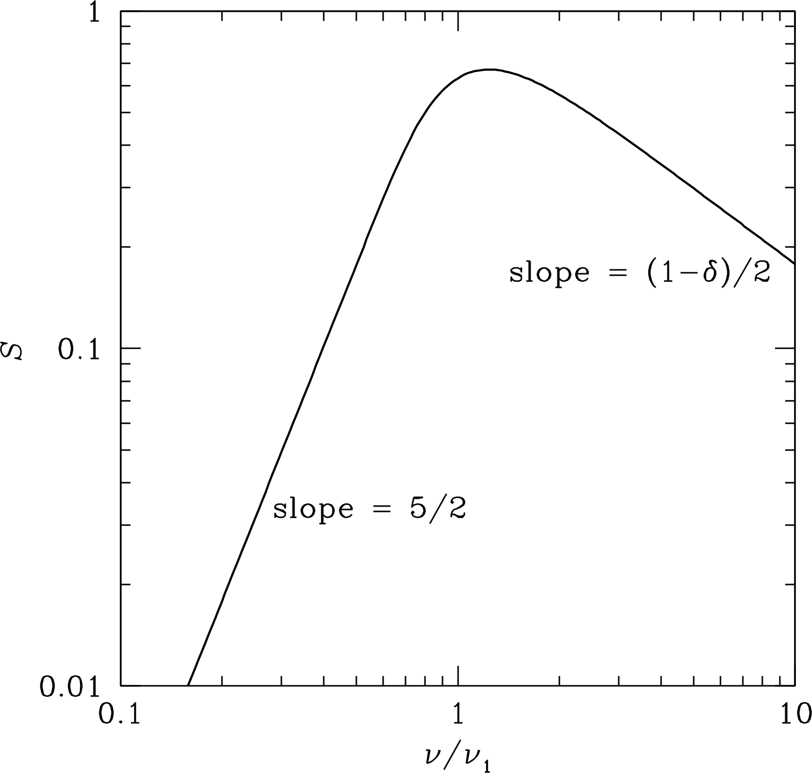
The full spectrum of a homogeneous cylindrical synchrotron source (Figure 5.7) is [78]
| (5.90) |
where is the frequency at which . Real astrophysical sources are inhomogeneous, so synchrotron self-absorption always yields slopes much lower than , as illustrated by Figure 5.8.
Substituting into Equation 5.85 yields an estimate of the magnetic field strength in a self-absorbed source whose brightness temperature has been measured at frequency :
| (5.91) |
For example, a self-absorbed radio source with observed brightness temperature K at GHz has a magnetic field strength
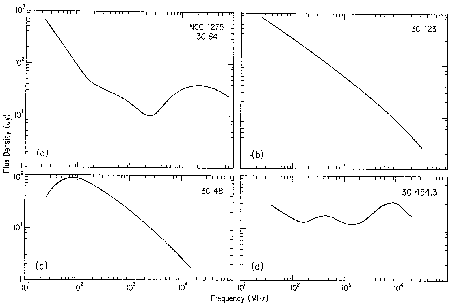
The spectra of celestial radio sources are more complex because real sources have nonuniform magnetic fields and electron energy distributions in geometrically complex structures. Representative spectra of powerful radio galaxies and quasars are illustrated in Figure 5.8.
Synchrotron radiation from cosmic-ray electrons accelerated by the supernova remnants of relatively massive () and short-lived ( yr) stars dominates the radio continuum emission of the nearby starburst galaxy M82 (Figure 8.13) at frequencies GHz (see the dot-dash line in Figure 2.24). Thermal emission (dashed line) from Hii regions ionized primarily by even more massive () and shorter-lived stars is strongest between about 30 and 200 GHz. At frequencies well below 1 GHz, free–free absorption flattens the overall spectrum.
5.4 Synchrotron Sources
5.4.1 Minimum Energy and Equipartition
The existence of a synchrotron source implies the presence of relativistic electrons with some energy density and a magnetic field whose energy density is . What is the minimum total energy in relativistic particles and magnetic fields required to produce a synchrotron source of a given radio luminosity
| (5.92) |
over the frequency range conventionally bounded by Hz and Hz?
The energy density of relativistic electrons in the energy range to is
| (5.93) |
where is the number density of electrons in the energy range to . Electrons with energy emit most of the radiation seen at frequency , so the electron energy corresponding to radiation at frequency satisfies
| (5.94) |
Thus the ratio of to can be written in terms of the energy limits:
| (5.95) |
where the synchrotron power emitted per electron is . For a power-law electron energy distribution ,
| (5.96) |
The energy limits and are both proportional to (Equation 5.94) so
| (5.97) |
Thus the electron energy density needed to produce a given synchrotron luminosity scales as
| (5.98) |
while the magnetic energy density is
| (5.99) |
The “invisible” cosmic-ray protons and heavier ions emit negligible synchrotron power but they still contribute to the total cosmic-ray particle energy. If the ion/electron energy ratio is , then the total energy density in cosmic rays is and the total energy density of both cosmic rays and magnetic fields is
| (5.100) |
Cosmic rays collected near the Earth have , but the value of in radio galaxies and quasars has not been measured.
The greatly differing dependences of and on means that the total energy density has a fairly sharp minimum near equipartition, the point at which (Figure 5.9).
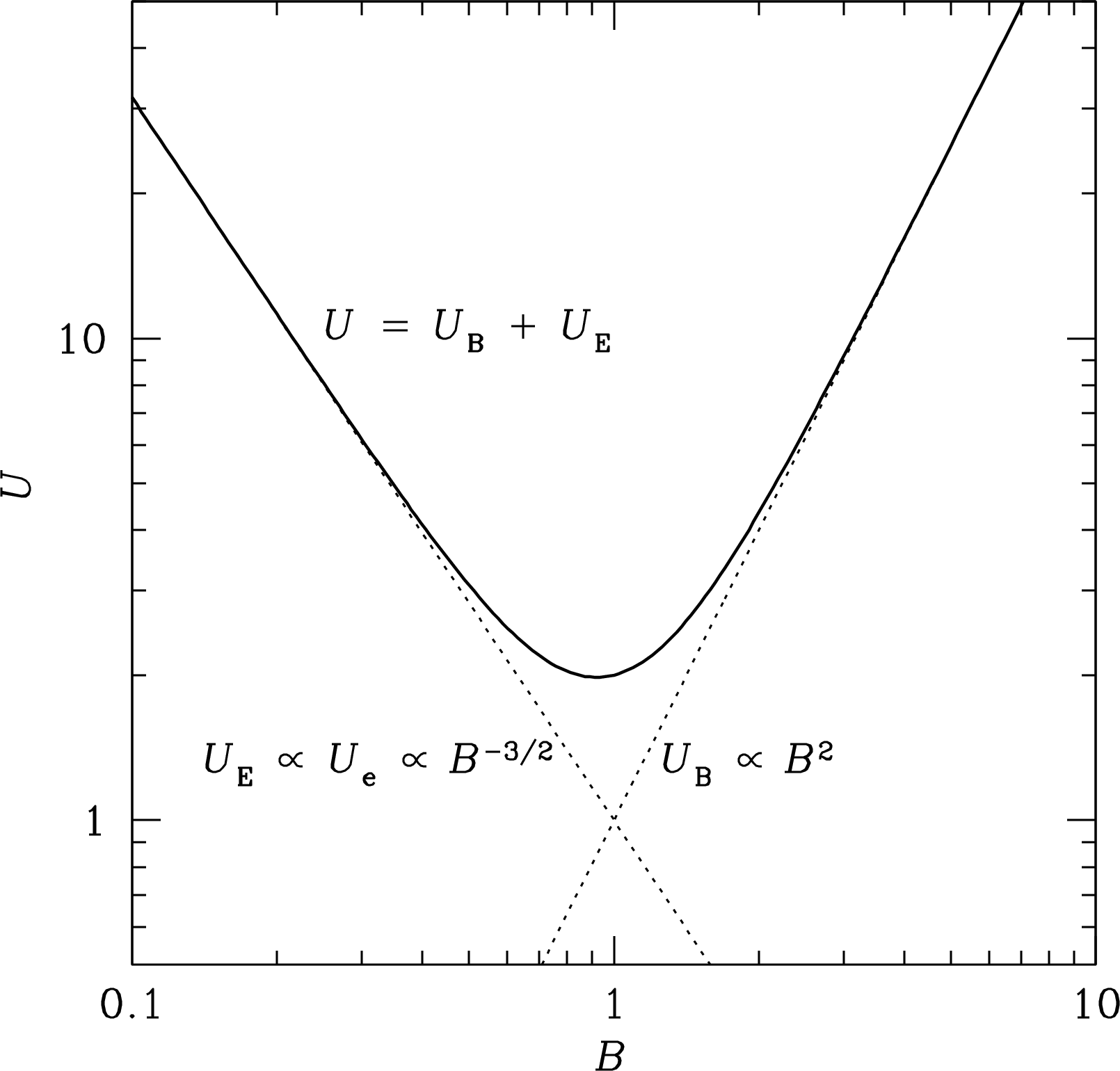
The minimum of the total energy density occurs at
| (5.101) |
The logarithmic derivative of the electron energy density is
| (5.102) |
so
| (5.103) |
The logarithmic derivative of the magnetic-field energy density is
| (5.104) |
so
| (5.105) |
Inserting Equations 5.103 and 5.105 into the minimum-energy Equation 5.101 gives
| (5.106) |
The ratio of cosmic-ray particle energy density to magnetic field energy that minimizes the total energy is
| (5.107) |
This ratio is nearly unity, so minimum energy implies (near) equipartition of energy: the total cosmic-ray energy density (including the energy of the nonradiating ions) is nearly equal to the total magnetic energy density . It is not known whether most synchrotron sources are in equipartition, but radio astronomers often assume so because
-
1.
it is physically plausible—systems with interacting components often tend toward equipartition;
-
2.
extragalactic radio sources with high luminosities and large volumes such as Cyg A have enormous total energy requirements even near equipartition; the “energy problem” is even worse otherwise;
-
3.
it eliminates an unknown parameter and permits estimates of the relativistic particle energies and the magnetic field strengths of radio sources with measured luminosities and sizes.
Getting the actual numerical values of the particle and magnetic-field energy densities from the synchrotron emission coefficient is a straightforward but tedious algebraic chore (Wilson et al. [116, Section 10.10]). The results (from Pacholczyk [78, p. 171]) are summarized in Equations 5.109 and 5.110. The functions and in these equations absorb the integrations from frequency to and the physical constants in Gaussian CGS units. The values of and are plotted in Figures 5.10 and 5.11.
For a spherical radio source with radius and magnetic field strength , the total magnetic energy is
| (5.108) |
The minimum-energy magnetic field strength for a source of radio luminosity is
| (5.109) |
and the corresponding total energy is
| (5.110) |
The synchrotron lifetime of a source is defined as the ratio of total electron energy to the energy loss rate from synchrotron radiation:
| (5.111) |
It approximates the lifetime of a synchrotron source if the primary loss mechanism is synchrotron radiation; if other loss mechanisms (e.g., inverse-Compton scattering) are significant, the actual source lifetime will be shortened. The synchrotron lifetime can be written as
| (5.112) |
5.4.2 The Eddington Luminosity Limit
The steady-state luminosity of an astronomical object of total mass is limited by the requirement that the outward radiation pressure cannot exceed the pull of gravity. Otherwise, radiation pressure would expel the outer layers of a star or disrupt accretion onto a compact object such as a black hole or neutron star. If the atmosphere of the star or the infalling material is primarily ionized hydrogen, the free electrons will Thomson-scatter outflowing radiation. The Thomson-scattering cross section is given by Equation 5.33. Each electron being pushed away by radiation pressure will drag along one proton () with it to maintain charge neutrality. Balancing the forces from radiation and gravity on each electron/proton pair at distance from the accreting object defines the Eddington luminosity:
| (5.113) |
Both forces are proportional to so
| (5.114) |
is proportional to the mass and independent of distance. In CGS units,
| (5.115) |
Normalized to “solar” units erg s and g,
| (5.116) |
| (5.117) |
For example, as the mass of a main-sequence star approaches , its luminosity approaches its Eddington luminosity. Very massive stars often have radiation-driven winds, and stars more massive than may not be stable. The Eddington limit doesn’t apply only to objects surrounded by ionized hydrogen, and analogs to the classical Eddington limit can be derived for other absorbers, such as interstellar dust. The ratio of the absorption cross section to mass for a typical dust grain is times larger than the ratio for ionized hydrogen, so the maximum luminosity-to-mass ratio of a dusty galaxy is times lower than given by Equation 5.117. Thus a supermassive black hole emitting at its Eddington limit for ionized hydrogen in the nucleus of a dusty galaxy may remove the dusty ISM if the galaxy mass is less than times the black-hole mass. Such radiative “feedback” processes may account for the observed mass ratio of galaxy bulges and their central black holes [37].
5.4.3 Application to the Luminous Radio Galaxy Cyg A
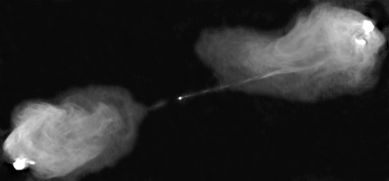
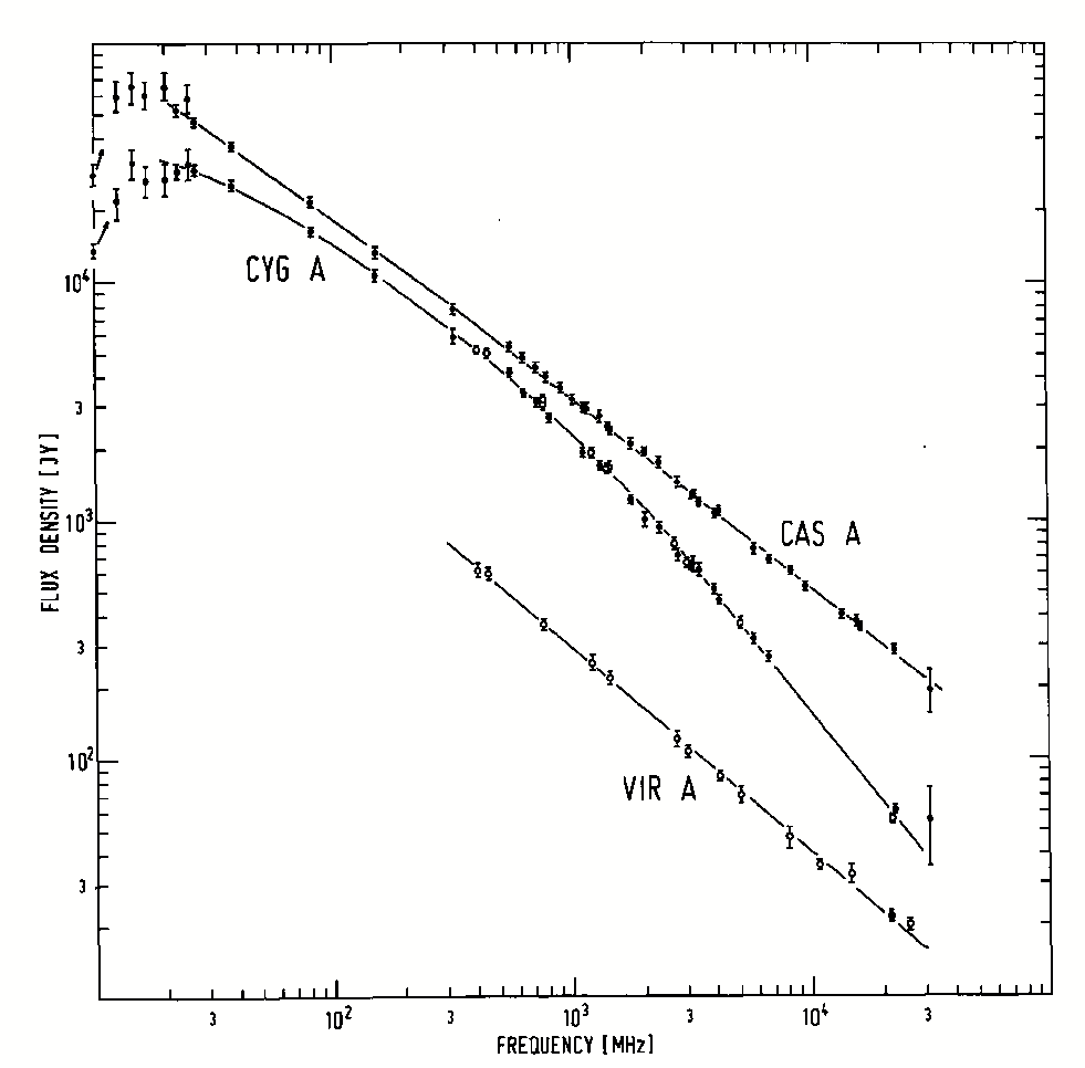
Cyg A is a luminous double radio source (Figure 5.12) in a peculiar galaxy at a distance Mpc. Its radio lobes have radii kpc, and the total flux density of Cyg A is
To estimate the total radio luminosity of Cyg A, first convert the data from “astronomical” units to Gaussian CGS units:
The spectral luminosity of Cyg A is
The total radio luminosity of Cyg A in the frequency range Hz to Hz is
In units of the bolometric solar luminosity , the radio luminosity of Cyg A is
The radio power from Cyg A exceeds the total power produced by all of the stars in our Galaxy.
The energy source for this radio emission is a compact object at the center of the host galaxy. The Eddington limit (Equation 5.117) yields a lower limit to its mass :
Note that the Eddington mass limit depends only on the instantaneous power emitted by the source, not on the total energy of the source, the source age, or any other indicator of its history.
The magnetic field strength that minimizes the total energy in the relativistic particles and magnetic fields implied by the luminous synchrotron source can be estimated with Equation 5.109. Approximate Cyg A (Figure 5.12) by two spherical lobes of radius kpc and luminosity each, where is the total luminosity of Cyg A:
The ion/electron energy ratio has not been measured in extragalactic radio sources such as Cyg A. The cosmic rays accelerated by a supermassive black hole might be primarily electrons and positrons. Electrons and positrons have equally large charge/mass ratios, so an electron–positron plasma would have . If electrons and protons are accelerated to the same velocity (same ), then the protons carry as much energy but emit almost nothing and . Fortunately, is only weakly dependent on —varying from 1 to changes from about 1 to 9:
| (5.118) | ||||
| (5.119) |
The minimum total energy (Equation 5.110) of Cyg A is twice the energy of each lobe:
| where is in the range of about 1 to 80; | ||||
| (5.120) | ||||
| (5.121) | ||||
Such large calculated energies can be confirmed observationally for sources in clusters of galaxies. Figure 8.15 shows that the radio source (red) in the galaxy cluster MS07356+7421 has displaced the X-ray emitting gas (blue) in a large volume. The gas pressure can be derived from the intensity of its the X-ray emission, and the total energy required to displace the gas is the product of the volume and the pressure [72].
This enormous energy implies an independent lower limit to the mass of the central object powering the radio source. Mass cannot be converted to energy with more than 100% efficiency, so the minimum mass needed to produce is
| (5.122) | ||||
| (5.123) |
This is a very conservative lower limit. Nuclear fusion can convert mass to energy with only % efficiency, so would be required for nuclear fusion in stars. Accretion onto a spinning black hole can yield efficiencies up to in theory, implying . Many authors assume that mass accreted by astronomical black holes is converted to energy with about 10% efficiency; this yields . The small size of the radio core measured by Very Long Baseline Interferometry (VLBI) and its observed flux variability on timescales of months to years combined with the large minimum masses estimated from the Eddington limit and the total energy of the radio lobes together make it difficult to avoid the conclusion that the compact, massive object powering the radio source is a supermassive black hole (SMBH). The adjective supermassive is used for black holes with , which is far more massive than the most massive stars, .
A lower limit to the age of the radio source Cyg A is the average synchrotron lifetime (Equation 5.111) of the relativistic electrons estimated by taking the ratio of the electron energy to the observed synchrotron luminosity:
| (5.124) | ||||
| (5.125) |
Because each electron radiates energy at a rate proportional to and the critical frequency is proportional to , the most energetic electrons emitting at the highest frequencies have the shortest lifetimes. The rapid depletion of high-energy electrons steepens the radio spectrum (Figure 5.13) of Cyg A frequencies higher than .
Suppose that new relativistic electrons are continuously injected with a power-law energy distribution
| (5.126) |
into a radio source. After a long time, electrons emitting at frequencies higher than will be depleted by radiative losses and these high-energy electrons will eventually reach an energy distribution . Consequently, the (negative) spectral index will be
| (5.127) |
at low frequencies and approach
| (5.128) |
at higher frequencies; that is, the high-frequency spectrum steepens by .
If the observed frequency of the spectral bend is high enough, the implied synchrotron lifetime of electrons with may be less than the time needed for new relativistic electrons to travel from the radio core to the emitting feature in a jet or lobe. This implies in situ acceleration—something outside the radio core (e.g., shocks in the jet) must replenish the supply of relativistic electrons. The radio spectrum of Vir A, the source in the galaxy M87, is straight to at least GHz (Figure 5.13), and this synchrotron emission extends to optical frequencies, so many of the cosmic rays must be accelerated in the bright shocked regions, not just near the black hole.
5.5 Inverse-Compton Scattering
The ambient radiation field is normally fairly isotropic in the rest frame of a synchrotron source. However, such a radiation field looks extremely anisotropic to each ultrarelativistic () electron producing the synchrotron radiation. Relativistic aberration (Section 5.3.1) causes nearly all ambient photons to approach within an angle rad of head-on (Figure 5.14). Thomson scattering of this highly anisotropic radiation systematically reduces the electron kinetic energy and converts it into inverse-Compton (IC) radiation by upscattering radio photons to become optical or X-ray photons. Inverse-Compton “cooling” of the relativistic electrons also limits the maximum rest-frame brightness temperature of an incoherent synchrotron source to K.
5.5.1 IC Power from a Single Electron
To derive the equations describing inverse-Compton scattering, first consider nonrelativistic Thomson scattering in the rest frame of an electron. If the Poynting flux (power per unit area) of a plane wave incident on the electron is
| (5.129) |
the electric field of the incident radiation will accelerate the electron, and the accelerated electron will in turn emit radiation according to Larmor’s equation. The net result is simply to scatter a portion of the incoming radiation, with no net transfer of energy between the radiation and the electron. The scattered radiation has power
| (5.130) |
where
| (5.131) |
is called the Thomson cross section (Equation 5.33) of an electron. In other words, the electron will extract from the incident radiation the amount of power flowing through the area and reradiate that power over the doughnut-shaped pattern given by Larmor’s equation. The scattered power can be rewritten as
| (5.132) |
where is the energy density of the incident radiation.
Next consider radiation scattering by an ultrarelativistic electron. Equation 5.132 is valid only in the primed frame instantaneously moving with the electron:
| (5.133) |
This nonrelativistic result needs to be transformed to the unprimed rest frame of an observer. Using the result (Equation 5.28) gives
| (5.134) |
To transform into , suppose that an electron moving with speed in the rest frame of the observer is hit successively by two low-energy photons approaching from an angle in the observer’s frame ( in the electron frame) from the -axis as shown in Figure 5.15. If the coordinates corresponding to the first and second photons hitting the electron (which is always located at ) are
| (5.135) |
in the observer’s frame, then the Lorentz transform Equation 5.12 gives the coordinates of these two events as
| (5.136) |
as shown in Figure 5.15.
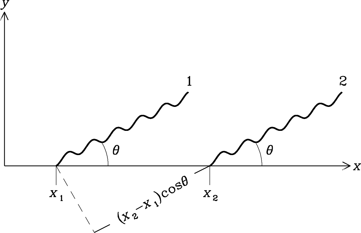
In the observer’s frame, the time elapsed between the arrival of these two photons at the plane (dashed line in Figure 5.15) normal to the direction of propagation is
| (5.137) | ||||
| (5.138) | ||||
| (5.139) |
where . The time between being hit by the two photons in the electron’s frame is so
| (5.140) |
The relativistic Doppler equation follows immediately from Equation 5.140. Let be the time between the arrivals of two successive cycles of a wave whose frequency is in the observer’s frame and in the moving frame. Then
| (5.141) |
or
| (5.142) |
In the electron’s frame, the frequency and energy of each photon are multiplied by . Moreover, the rate at which successive photons arrive is multiplied by the same factor. If is the photon number density in the observer’s frame, then . In the observer’s frame, the radiation energy density is
| (5.143) |
In the electron’s frame
| (5.144) |
Thus the transformation between and depends on the angle between the direction of the photons in the plane wave and the direction of the electron motion.
For a radiation field of total energy density that is isotropic in the observer’s frame, the energy density per unit solid angle is and the total energy density in the electron frame can obtained by integrating Equation 5.144 over all directions:
| (5.145) |
where is the azimuthal angle around the -axis. Thus
| (5.146) |
To evaluate this integral, substitute so and eliminate in favor of :
| (5.147) | ||||
| (5.148) |
Recall that so
| (5.149) |
Substituting this result for into Equation 5.134 yields
| (5.150) |
for the total power radiated after inverse-Compton upscattering of low-energy photons. The initial power of these photons was , so the net power added to the radiation field by inverse-Compton scattering is
| (5.151) |
Replacing by gives the final result
| (5.152) |
for the net inverse-Compton power gained by the radiation field and lost by the electron. Dividing by the corresponding synchrotron power (Equation 5.42)
| (5.153) |
reveals the remarkably simple ratio of IC to synchrotron radiation losses:
| (5.154) |
The IC loss is proportional to the radiation energy density and the synchrotron loss is proportional to the magnetic energy density. Note that synchrotron and inverse-Compton losses have the same electron-energy dependence (), so their effects on radio spectra (Equation 5.128) are indistinguishable.
5.5.2 The IC Spectrum of a Single Electron
What is the spectrum of the inverse-Compton radiation? Suppose the ambient radiation field in the observer’s frame contains only photons of frequency , and consider scattering by a single electron moving with ultrarelativistic velocity along the -axis. In the inertial frame moving with the electron, relativistic aberration causes most of the photons to approach nearly head-on. The relativistic Doppler Equation 5.142 gives the frequency in the electron frame of a photon approaching near the -axis (); it is
| (5.155) |
In the electron frame, Thomson scattering produces radiation with the same frequency as the incident radiation: the scattered photons have . In the observer’s frame, relativistic aberration beams the scattered photons in the direction of the electron’s motion, and the frequency of radiation scattered nearly along the -direction () is given by the relativistic Doppler formula:
| (5.156) |
In the ultrarelativistic limit ,
| (5.157) |
This is the maximum frequency of the upscattered radiation in the observer’s frame.
Oblique collisions () result in lower frequencies . For an isotropic radiation field in the observer’s frame, the average energy of scattered photons equals the average scattered power per electron divided by , the number of photons scattered per second per electron. This rate is the scattered power divided by the photon energy in the observer’s frame, or
| (5.158) |
Thus
| (5.159) |
and the average frequency of upscattered photons is
| (5.160) |
For example, isotropic radio photons at GHz, IC scattered by electrons having , will be upscattered to an average frequency
corresponding to X-ray radiation. The principal astronomical effect of inverse Compton scattering is to drain energy from cosmic-ray electrons that produce radio radiation and use it to produce X-ray radiation instead.
Because the maximum frequency (Equation 5.157) is only three times the average frequency (Equation 5.160), the IC spectrum must be sharply peaked near the average frequency. The detailed Compton-scattering spectrum resulting from an isotropic single-frequency radiation field has been calculated (Blumenthal and Gould [13]; see also Pacholczyk [78]). It is indeed sharply peaked just below the maximum , as shown in Figure 5.16.
This spectrum is even more peaked than the synchrotron spectrum of monoenergetic electrons. Therefore it is not necessary to use the detailed Compton-scattering spectrum of monoenergetic electrons to calculate the inverse-Compton spectrum of an astrophysical source containing a power-law distribution of relativistic electrons. If the electron-energy distribution is , the inverse-Compton spectrum will also be a power law with spectral index
| (5.161) |
which is the same spectral index that Equation 5.79 gives for synchrotron radiation emitted by the same power-law distribution of electron energies.
5.5.3 Synchrotron Self-Compton Radiation
Synchrotron self-Compton radiation results from inverse-Compton scattering of synchrotron radiation by the same relativistic electrons that produced the synchrotron radiation. Equation 5.154,
| (5.162) |
implies that multiplying the density of relativistic electrons by some factor multiplies both the synchrotron power and its contribution to by , so the synchrotron self-Compton power is proportional to .
The self-Compton radiation also contributes to and leads to significant second-order scattering as the synchrotron self-Compton contribution to approaches the synchrotron contribution in compact sources. This runaway positive feedback is a very sensitive function of the source brightness temperature, so inverse-Compton losses very strongly cool the relativistic electrons if the source brightness temperature exceeds K in the rest frame of the source. Radio sources with brightness temperatures significantly higher than
| (5.163) |
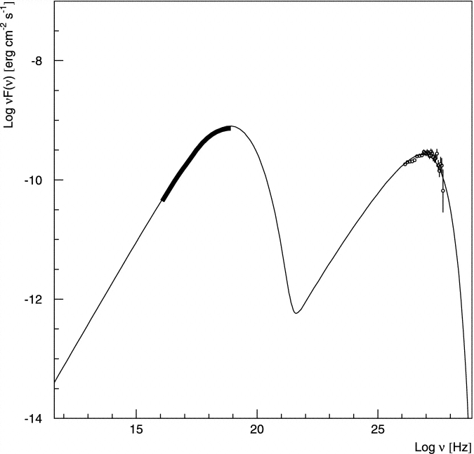
in the observer’s frame are either Doppler boosted or not incoherent synchrotron sources (e.g., pulsars are coherent radio sources). The active galaxy Markarian 501 emits strong synchrotron self-Compton radiation and the radio emission approaches this rest-frame brightness limit for incoherent synchrotron radiation. The synchrotron and synchrotron self-Compton spectra of Mrk 501 are shown in Figure 5.17.
5.6 Extragalactic Radio Sources
5.6.1 Relativistic Bulk Motion
The results above apply only to radio-emitting plasmas that are not moving relativistically with respect to the observer. Bright radio-source components (discrete regions of enhanced brightness) are often seen to move with apparent transverse velocities exceeding the speed of light. This illusion of superluminal velocities can occur if the components are moving obliquely toward the observer with relativistic speeds, as shown in Figure 5.18.
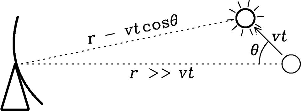
Suppose the radio-emitting component is moving toward the observer with constant speed at an angle from the line of sight. Consider two “events” in the moving component, the first occurring a distance from the observer at time , and the second at time . Radiation from the first and second events will be received at times
| (5.164) |
respectively. The difference between these times is
| (5.165) |
The apparent transverse velocity of the moving component is the actual transverse distance covered in time divided by the apparent time interval :
| (5.166) | |||
| (5.167) |
For every speed there is an angle that maximizes . That angle satisfies
| (5.168) | |||
| (5.169) |
Thus
| (5.170) |
and
| (5.171) |
Inserting and into Equation 5.167 for yields the highest apparent transverse speed of a source whose actual speed is :
| (5.172) |
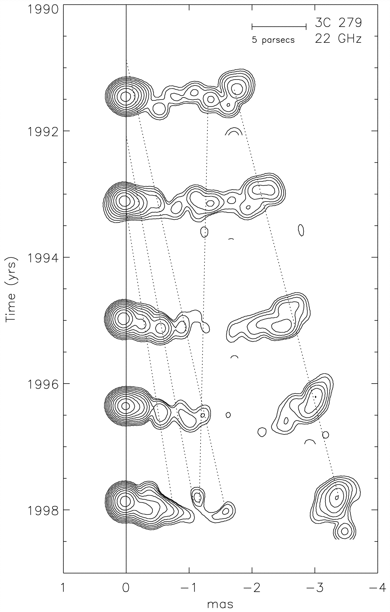
Figure 5.19 shows five successive high-resolution radio images of the quasar 3C 279. The bright component at the left is taken to be the fixed radio core, and the bright spot at the right appears to have moved 25 light years across the plane of the sky between 1991 and 1998, for an apparently superluminal motion of 25 light years in 7 years: . What is the minimum component speed consistent with these images? What is the corresponding angle between that motion and the line of sight? From the results above,
| (5.173) |
so
| (5.174) | ||||
| (5.175) |
The corresponding is given by
| (5.176) | |||
| (5.177) |
The relativistic Doppler formula (5.142) relates the frequency emitted in the component frame to the observed frequency . Note that we have replaced by () radians in the current analysis by calling it the angle between the line of sight and the velocity of an approaching component, so
| (5.178) |
where now corresponds to a radio component moving directly toward the observer. The quantity
| (5.179) |
is called the Doppler factor. If , there is a transverse Doppler shift
| (5.180) |
The transverse Doppler shift has no nonrelativistic counterpart because the source has no component of velocity parallel to the line of sight; it exists only because moving clocks run slower by a factor . The Doppler factors associated with a given source speed range from
| (5.181) |
for directly receding ( rad) sources to
| (5.182) |
for directly approaching () sources. For example, the ratio of the observed frequency to the emitted frequency in 3C 279 (, ) is
The observed flux density of a relativistically moving component emitting isotropically in its rest frame depends critically on its Doppler factor . The exact amount of Doppler boosting caused by relativistic beaming is somewhat model dependent [101] but probably lies in the range
| (5.183) |
where would be the observed flux density if the source were stationary and is the (negative) spectral index. If , then depending on the angle . Relativistic components approaching at angles can easily be boosted by factors compared with components moving in the sky plane or away from us. For example, the approaching jet of 3C 279 ( and ) is Doppler boosted by
The receding counterjet is dimmed by a comparable factor, so the jet/counterjet observed flux-density ratio of 3C 279 is probably .
Doppler boosting strongly favors approaching relativistic jets and components and discriminates against those with in flux-limited samples of compact radio sources. Radio quasars aren’t isotropic candles spread throughout the universe; they are beamed flashlights. The brightest aren’t always the most luminous; they are just pointing in our direction. For every flashlight we see, there are many others in the same volume of space that we don’t see simply because they are not pointing at us.
The fact that the two lobes of very extended radio sources such as Cyg A (Figure 5.12) and 3C 348 (Figure 8.14) typically have flux ratios indicates that the lobes are moving outward with speeds . The radio jets feeding nearly equal lobes often appear quite unequal, with one jet being very strong and the other undetectable. The jets of very luminous sources often terminate in bright hotspots in the lobes.
Because the jets feed the lobes, the lobe symmetry suggests that the jets are intrinsically similar, but the approaching jet is boosted while the receding counterjet is dimmed. Another feature of many radio jets is gaps near the core. If jets start out relativistic at the core and are inclined by more than from the line of sight, both will be Doppler dimmed. If they proceed with constant but gradually decelerate as they move away from the core, one or both may become visible beyond the point where .
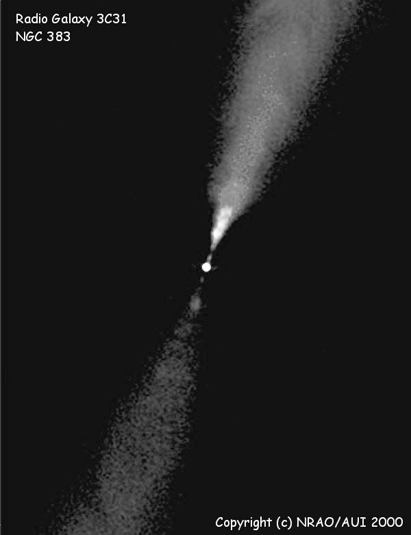
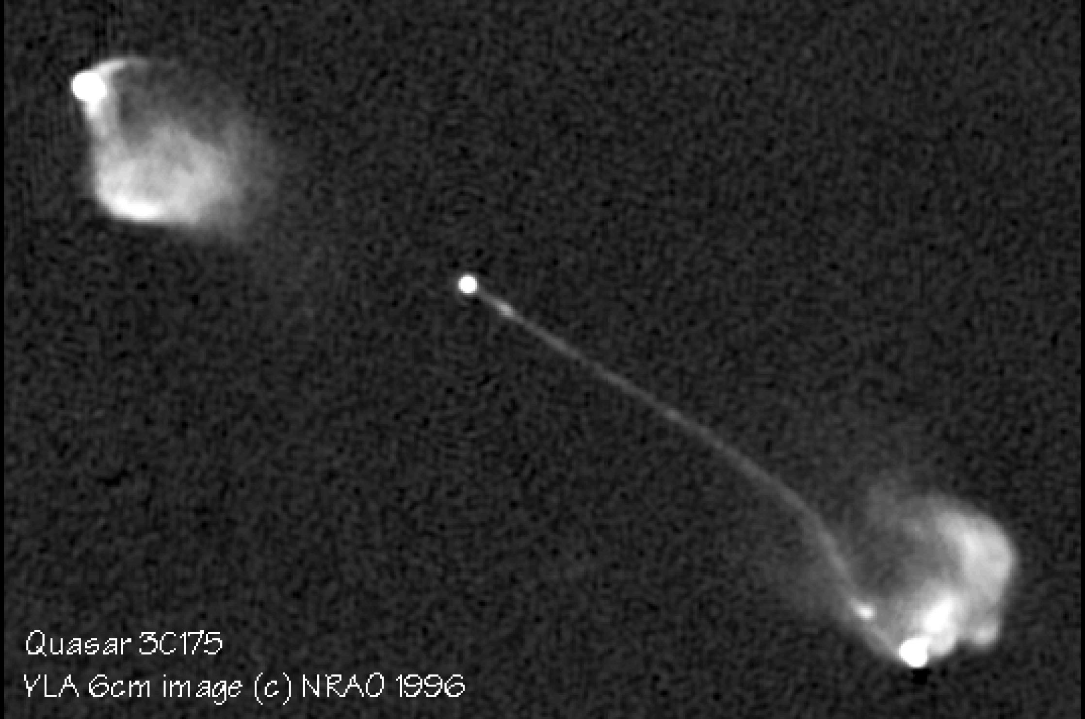
Extragalactic radio sources with jets and lobes can be divided into two morphological classes: (1) those, like 3C 31 (Figure 5.20), that appear to fade away at large distances from the center and (2) sources with edge-brightened lobes, like 3C 175 (Figure 5.21). Such sources are called FR I and FR II sources, respectively, after Fanaroff and Riley [38], who first made such classifications and noted that FR I sources are usually less luminous than FR II sources, with the dividing line being at 1.4 GHz. FR I sources generally have lower equipartition energy densities and hence lower equipartition pressures. The jets of FR I sources are fairly symmetric at distances greater than several kpc from the cores, suggesting that the low-luminosity jets are quickly decelerated to nonrelativistic speeds. The low-energy FR I jets are easily influenced by ambient matter. Low-luminosity galaxies moving through the intracluster medium of a cluster of galaxies frequently have bent head-tail radio morphologies similar to the wake of a moving boat.
5.6.2 Unified Models
The combination of orientation-dependent beaming and obscuration by dust has led to various unified models (Figure 5.22) of active galactic nuclei (AGN).
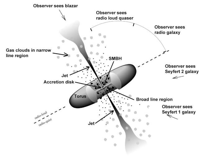
These models attribute some or all of the differences between observationally different objects to the inclinations of their jets relative to the line of sight. If the inclination is small, the base of the approaching jet will be strongly Doppler boosted, and the compact optical broad-line region and inner accretion disk will not be obscured by the larger dusty accretion torus lying in a plane normal to the jet. The observed radio emission will be dominated by a one-sided jet that may be variable in intensity and apparently superluminal. Thermal emission from the inner parts of the accretion disk may be visible as a big blue bump in the optical/UV spectrum, and Doppler-broadened emission lines from the small ( pc) broad-line region will not be obscured. If the optical AGN emission is much brighter than the starlight of the host galaxy, the object will be called a quasi-stellar object (QSO), but otherwise a Seyfert I galaxy. In extreme cases, optical synchrotron emission may dominate the big blue bump and emission lines. Objects with lineless power-law optical spectra are often called BL Lac objects after their prototype BL Lacertae, which was originally thought to be a Galactic star (hence the constellation name). If the inclination angle is larger than about 45 degrees, the optical core may be obscured by the dusty torus and highly relativistic radio jets may be Doppler dimmed, and we will see either a double-lobed radio galaxy or a Seyfert II galaxy (a Seyfert galaxy with only the narrow emission lines directly visible). The ongoing debate over unified models is not about whether relativistic beaming and dust obscuration affect the appearance of AGNs, but how much.
5.6.3 Radio Emission from Normal Galaxies
The radio emission from a normal galaxy is not powered by an AGN. The continuum radio emission from normal galaxies is dominated by a combination of
-
1.
free–free emission from Hii regions ionized by massive () main-sequence stars, and
-
2.
synchrotron radiation from cosmic-ray electrons, most of which were accelerated in the supernova remnants (SNRs) of massive () stars.
Stars more massive than have main-sequence lifetimes yr, much less than the yr age of our Galaxy. Also, the synchrotron lifetimes of cosmic-ray electrons in the typical interstellar magnetic field are yr. Thus the current radio continuum emission from normal galaxies is an extinction-free tracer of recent star formation, unconfused by emission from older stars. The radio emission is roughly coextensive with the locations of star formation, spanning the stellar disks of most spiral galaxies.
Massive stars form by gravitational collapse in dusty molecular clouds. The dust absorbs most of their visible and ultraviolet radiation, is heated to temperatures of several tens of K, and reemits the input energy at far-infrared (FIR) wavelengths m. The molecular clouds are not opaque at FIR wavelengths, so FIR luminosity is a good quantitative measure of the current star-formation rate. Remarkably, the radio luminosities of normal galaxies are very tightly correlated with their FIR luminosities.
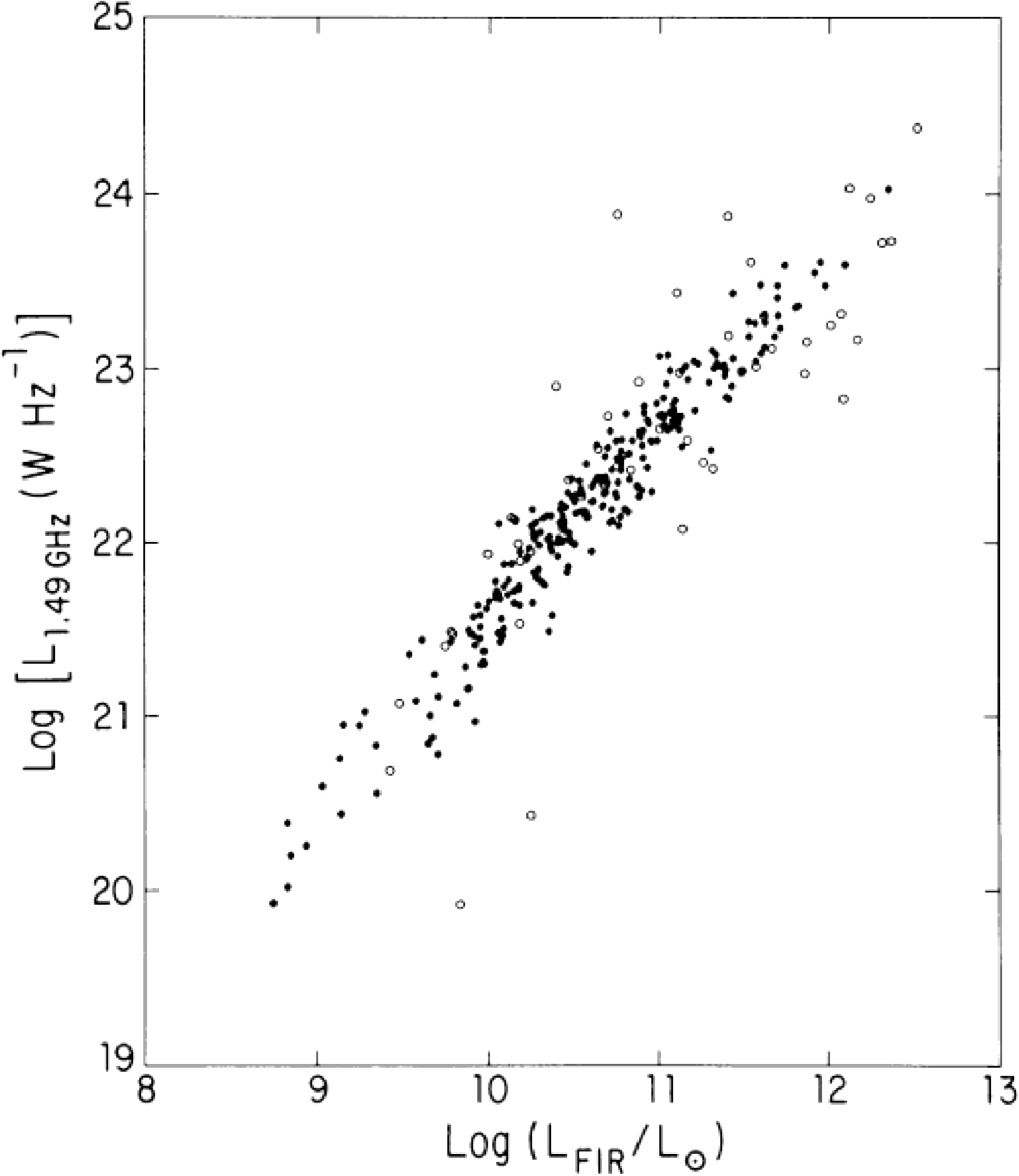
The physical origin of this famous FIR/radio correlation (Figure 5.23) is poorly understood, particularly at low frequencies where most of the radio emission is synchrotron radiation. It is not surprising that the FIR and free–free radio fluxes would be correlated because both are roughly proportional to the ionizing luminosities of massive young stars. However, free–free emission accounts for only a small fraction of the total radio luminosity at low frequencies GHz. The FIR/radio spectrum of the nearby starburst galaxy M82 (Figure 2.24) is typical.
At GHz, about 90% of the radio flux is produced by synchrotron radiation, yet the FIR/radio luminosity ratio is confined to a very narrow range. If the star-formation rate (SFR) in a galaxy is fairly constant on timescales longer than yr, then the number of young SNRs would be proportional to the present number of massive stars, so it is plausible that the current production rate of cosmic-ray electrons is proportional to the current star-formation rate. However, most of the synchrotron radiation from normal galaxies does not originate in the SNRs themselves, but rather comes from cosmic-ray electrons that have diffused into the interstellar medium (ISM). The power radiated by each electron is proportional to the magnetic energy density in the ISM. The equipartition fields in normal galaxies range from very low values to G in a typical spiral galaxy like ours, to G in M82 and up to G in a particularly compact and luminous starburst galaxy such as Arp 220. Thus the power radiated by each cosmic-ray electron must vary by up to several orders of magnitude from one galaxy to another, yet all of these galaxies obey the same FIR/radio correlation.
The calorimeter model [112] was devised to explain how the FIR/radio ratio could be independent of . The total radio energy radiated by each electron might be independent of if the lifetime of the electron is proportional to . Thus, a cosmic-ray electron in a strong magnetic field radiates a high power for a short time, while one in a weak magnetic field radiates a lower power for a proportionately longer time. For a given production rate of cosmic-ray electrons, the average synchrotron power will then be independent of . The calorimeter model works well to explain the FIR/radio correlation so long as the fraction of the electron energy going into synchrotron radiation is about the same in all normal galaxies. However, there are many other energy-loss channels. One is inverse-Compton scattering off the cosmic microwave background, starlight, FIR radiation, etc. Another is diffusion out of the magnetic field of a galaxy—some electrons escape silently into intergalactic space. Electrons may also lose energy by colliding with atoms in the ISM.
Galaxy–galaxy collisions can trigger intense starbursts (star-formation episodes so intense that they will deplete the available ISM on timescales much shorter than yr) within several hundred parsecs of the centers of galaxies and produce compact central sources. The radiation energy density in a compact starburst galaxy such as Arp 220 can reach , yet Arp 220 still obeys the FIR/radio correlation. The fact that inverse-Compton cooling doesn’t seriously deplete the population of synchrotron-emitting electrons sets a lower limit to the interstellar magnetic energy density via Equation 5.154. This limit is in Arp 220 [29].
Despite its uncertain theoretical basis, the FIR/radio correlation makes radio continuum emission from normal galaxies a very useful, quantitative, and extinction-free indicator of the rate at which massive stars are being formed. The rate (measured in units of solar masses per year) at which stars with masses are formed in a galaxy can be estimated from the thermal (free–free) and nonthermal (synchrotron) spectral luminosities by the following equations [30]:
| (5.184) |
| (5.185) |
5.6.4 Extragalactic Radio-Source Populations and Cosmological Evolution
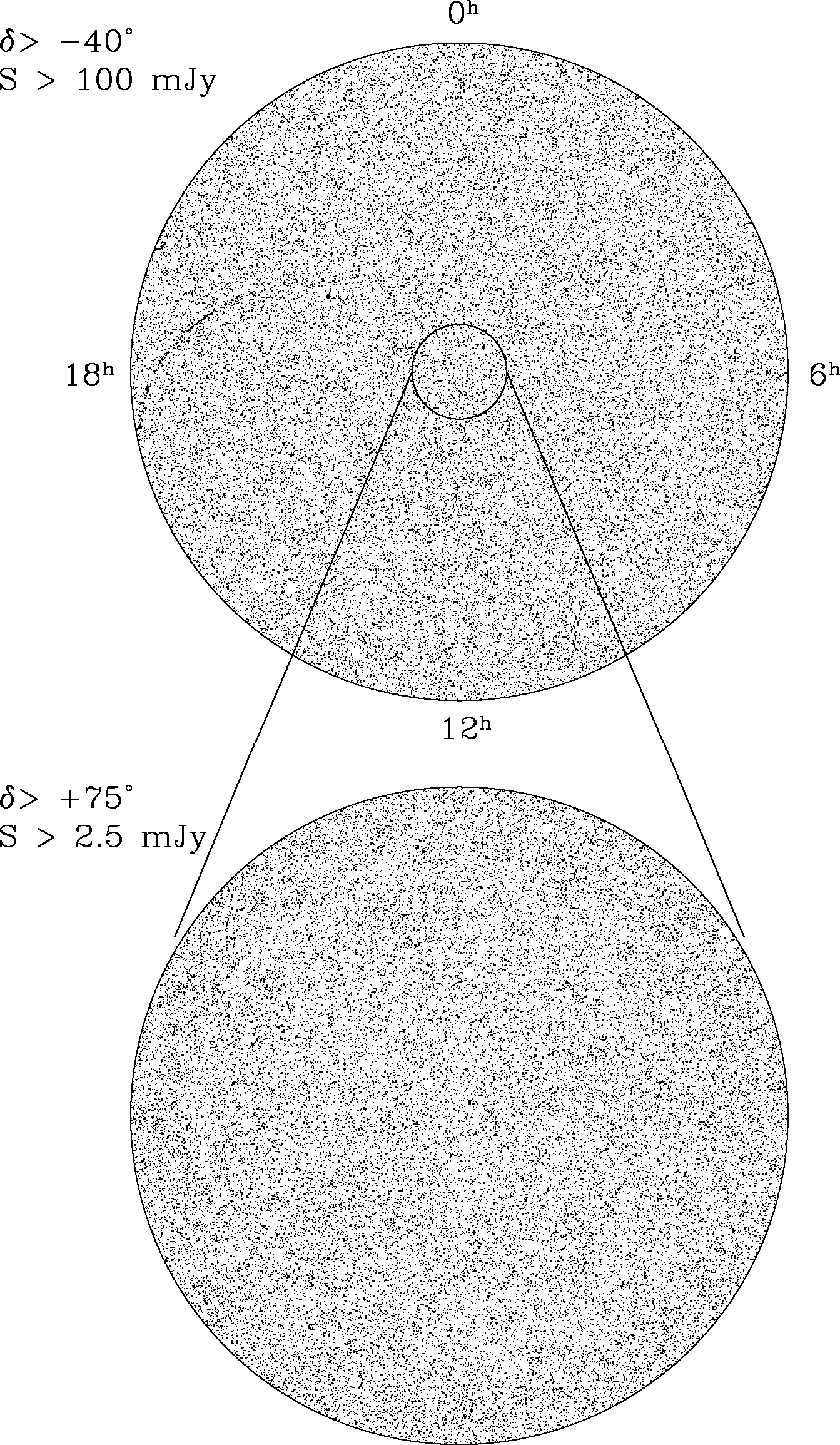
Surveys of discrete radio sources have been made over large areas of the sky and at many frequencies ranging from 38 MHz to 857 GHz. The most extensive sky survey is the NRAO VLA Sky Survey (NVSS) [28], which covers the whole sky north of declination (latitude on the celestial sphere) and detected nearly sources stronger than mJy at 1.4 GHz. Extremely sensitive sky surveys covering much smaller areas have reached flux densities Jy. Sources detected by blind surveys covering representative areas of sky give us an unbiased statistical sample of the radio-source population.
The distribution of discrete sources on the sky is extremely isotropic, as shown in Figure 5.24. This isotropy indicates that nearly all radio sources in a flux-limited sample are extragalactic—the center of our Galaxy is barely visible as the curved band at the left of the upper panel. A similar plot of the brightest galaxies selected at optical or near-infrared wavelengths is much clumpier than the radio plots because galaxies cluster on scales Mpc in size. The reason for this difference is that the strongest extragalactic radio sources are much farther away than the optically brightest galaxies. Radio galaxies are at least as clustered as optical galaxies, but the average distance between radio galaxies is so much greater than 10 Mpc that their clustering can be detected only by sensitive statistical tests. Indeed, the distribution of radio sources on the sky is so uniform that the small (%) dipole anisotropy in source density caused by Doppler boosting from the Earth’s motion relative to the frame defined by distant galaxies has been detected. The velocity of the Earth deduced from this anisotropy is consistent with the motion deduced from the corresponding anisotropy in the cosmic microwave background radiation produced by the hot big bang [11].
Only a small fraction (%) of radio sources in a flux-limited sample are closer than about 100 Mpc. By identifying those sources with bright galaxies and determining their Hubble distances, we can determine the space density of nearby radio sources as a function of radio spectral luminosity; this is called the local luminosity function. The local luminosity function can be further refined by specifying separately the space densities of radio sources powered by AGN and those powered by star-forming galaxies containing Hii regions, SNRs, etc. (Figure 5.25).
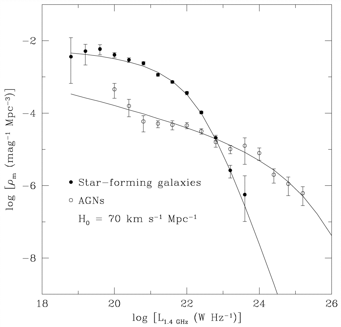
In a given volume of space, radio sources in star-forming galaxies outnumber radio galaxies containing AGN by an order of magnitude. However, the rarer AGN produce all of the most luminous sources, so they account for slightly over half of all radio emission produced by discrete sources.
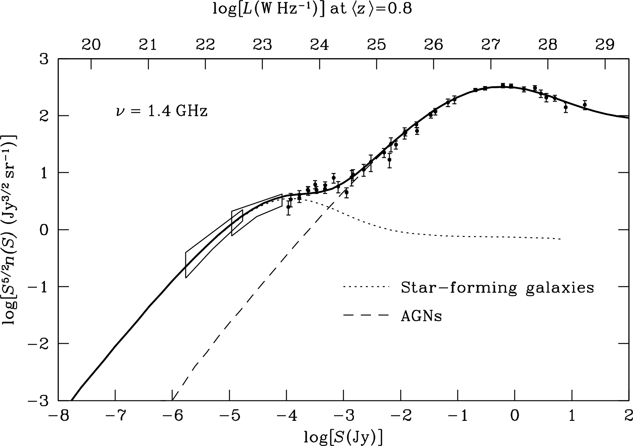
If we assume that the comoving space density of radio sources in the expanding universe is independent of time, we can use the local luminosity function to calculate the total number of radio sources per steradian of sky as a function of flux density. The resulting source counts are usually tabulated in differential form: is the number of sources per sr with flux densities between and . In a static Euclidean universe, the flux density of any source at distance is proportional to , and the volume enclosed by a sphere is proportional to , so the integral number of sources stronger than any given flux density should be proportional to and the differential number per unit flux density should be . Plotting the normalized differential source count as a function of should yield a horizontal line in a static Euclidean universe.
The actual plot for sources selected at 1.4 GHz is shown in Figure 5.26. The source counts are not consistent with a static Euclidean universe, so most radio sources cannot be “local” extragalactic sources. In an expanding universe with a constant comoving source density, distant sources will be Doppler dimmed and the normalized source counts should decline monotonically at low flux densities. This is not the case either; the normalized counts have a clear maximum near mJy. This peak indicates that radio sources must be evolving on cosmological timescales; that is, their comoving space density varies with time and was higher at some time in the past. The discovery of radio-source evolution was used as evidence against the steady-state model of the universe [100], years before the discovery of the cosmic microwave background radiation decisively confirmed the hot big-bang model.
Detailed models consistent with the local luminosity function, radio source counts, and redshift distributions of radio sources identified with galaxies and quasars have been constructed to measure the amount of evolution. The results are actually quite simple: cosmological evolution is so strong that most radio sources in flux-limited samples have redshifts near the median . To radio astronomers, the universe looks like a nearly hollow spherical shell centered on the Earth. This observation does not conflict with the Copernican principle, which states that the Earth is not in a special position at the center of the universe; it requires only that the universe evolve with time. Most radio sources seen today have distances of 5 to light years, and their dominance reflects the higher AGN and star-formation activity of 5 to 10 Gyr ago. For sources in a thin shell, there is little correlation between flux density and average distance; rather, flux density is more closely correlated with absolute luminosity as shown by labels on the lower and upper abscissae in Figure 5.26. Consequently, radio-loud AGNs in radio galaxies and quasars (dashed curve in Figure 5.26) account for most sources stronger than mJy at 1.4 GHz, and the numerous but less luminous star-forming galaxies (dotted curve in Figure 5.26) dominate the microJy radio-source population.