Essential Radio Astronomy 6 Pulsars 8 Color Plates

Chapter 7 Spectral Lines

7.1 Introduction

Spectral lines are narrow ( $\Delta\nu\ll\nu$ ) emission or absorption features in the spectra of gaseous and ionized sources. Examples of radio spectral lines include recombination lines of ionized hydrogen and heavier atoms, rotational lines of polar molecules such as carbon monoxide (CO), and the $\lambda=21$ cm hyperfine line of interstellar Hi.

Spectral-line emission and absorption are intrinsically quantum phenomena. Classical particles and waves are idealized concepts like infinitesimal points or perfectly straight lines in geometry; they don’t exist in the real world. Some things are nearly waves (e.g., radio waves) and others are nearly particles (e.g., electrons), but all share characteristics of both particles and waves. Unlike idealized waves, real radio waves do not have a continuum of possible energies. Instead, electromagnetic radiation is quantized into photons whose energy is proportional to frequency: $E=h\nu$ . Unlike idealized particles, real particles of momentum $p$ are associated with waves whose De Broglie wavelength is $\lambda=h/p$ . An electron’s stable orbit about the nucleus of an atom shares a property with standing waves: its circumference must equal an integer number of wavelengths. Planck’s constant $h\approx 6.62607\times 10^{-27}$ erg s in these two equations is a quantum of action whose dimensions are (mass $\times$ length ${}^{2}\times$ time ${}^{-1}$ ), the same as (energy $\times$ time) or (angular momentum) or (length $\times$ momentum). Although $h$ has dimensions of energy $\times$ time, physically acceptable solutions (the wave functions and their derivatives must be finite and continuous) to the time-independent Schrödinger equation exist only for discrete values of the total energy, so spectral lines have definite frequencies resulting from transitions between discrete energy states. A second quantum effect important to spectral lines, particularly at radio wavelengths where $h\nu\ll kT$ , is stimulated emission (Section 7.3.1). Fortunately, the fundamental characteristics of radio spectral lines from interstellar atoms and molecules can be derived from fairly simple applications of quantum mechanics and thermodynamics.

Spectral lines are powerful diagnostics of physical and chemical conditions in astronomical objects. Their rest frequencies identify the specific atoms and molecules involved, and their Doppler shifts measure radial velocities. These velocities yield the redshifts and Hubble distances of extragalactic sources, plus rotation curves and radial mass distributions for resolved galaxies. Collapse speeds, turbulent velocities, and thermal motions contribute to line broadening in Galactic sources. Temperatures, densities, and chemical compositions of Hii regions, dust-obscured dense molecular clouds, and diffuse interstellar gas are also constrained by spectral-line data. Radio spectral lines have some unique characteristics:

1.

Their “natural” line widths are much smaller than Doppler-broadened line widths, so gas temperatures and very small changes in radial velocity can be measured.
2.

Stimulated emission is important because $h\nu\ll kT$ . This causes line opacities to vary as $T^{-1}$ and favors the formation of natural masers.
3.

The ability of radio waves to penetrate dust in our Galaxy and in other galaxies allows the detection of line emission emerging from dusty molecular clouds, protostars, and molecular disks orbiting AGNs.
4.

Frequency (inverse time) can be measured with much higher precision than wavelength (length), so very sensitive searches for small changes in the fundamental physical constants over cosmic timescales are possible.

Although the interstellar medium (ISM) of our Galaxy is dynamic, it tends toward a rough pressure equilibrium because mass motions with speeds up to the speed of sound try to reduce pressure gradients. Temperatures equilibrate more slowly, so there are wide ranges of temperature $T$ and particle number density $n$ consistent with a given pressure $p$ and the ideal gas law

\boxed{p=nkT.}

(7.1)

Typical ISM pressures lie in the range $p/k=nT\sim 10^{3}$ – $10^{4}\mathrm{~{}cm}^{-3}\mathrm{~{}K}$ [58]. Radiative cooling by spectral-line emission depends strongly on temperature, so most of the ISM exists in several distinct phases having comparable pressures but quite different temperatures:

1.

cold (10s of K) dense molecular clouds
2.

cool ( $\sim 10^{2}$ K) neutral Hi gas
3.

warm ( $\sim 5\times 10^{3}$ K) neutral Hi gas
4.

warm ( $\sim 10^{4}$ K) ionized Hii gas
5.

hot ( $\sim 10^{6}$ K) low-density ionized gas (in bubbles formed by expanding supernova remnants, for example)

All but the hottest phase are sources of radio spectral lines.

7.2 Recombination Lines

7.2.1 Recombination Line Frequencies

The semiclassical Bohr atom (Figure 7.1) contains a nucleus of protons and neutrons around which one or more electrons move in circular orbits. The nuclear mass $M$ is always much greater than the sum of the electron masses $m_{\mathrm{e}}$ , so the nucleus is nearly at rest in the center-of-mass frame. The wave functions of the electrons have De Broglie wavelengths

\lambda=\frac{h}{p}=\frac{h}{m_{\mathrm{e}}v},

(7.2)

where $p$ is the electron’s momentum and $v$ is its speed. Only those orbits whose circumferences equal an integer number $n$ of wavelengths correspond to standing waves and are permitted. Thus the Bohr radius $a_{n}$ of the $n$ th permitted electron orbit satisfies the quantization rule

2\pi a_{n}=n\lambda=\frac{nh}{m_{\mathrm{e}}v},

(7.3)

where the number $n$ is called the principal quantum number. The requirement that

a_{n}=\frac{nh}{2\pi m_{\mathrm{e}}v}=\frac{n\hbar}{m_{\mathrm{e}}v}

(7.4)

implies that the orbital angular momentum $L=m_{\mathrm{e}}va_{n}=n\hbar$ is an integer multiple of the reduced Planck’s constant $\hbar\equiv h/(2\pi)$ . The relation between $a_{n}$ and $v$ is determined by the balance of Coulomb and centrifugal forces on electrons in circular orbits. For a hydrogen atom,

\frac{e^{2}}{a_{n}^{2}}=\frac{m_{\mathrm{e}}v^{2}}{a_{n}}.

(7.5)

Equations 7.4 and 7.5 can be combined to eliminate $v$ and solve for $a_{n}$ in terms of $n$ and physical constants:

\boxed{a_{n}=\frac{n^{2}\hbar^{2}}{m_{\mathrm{e}}e^{2}}.}

(7.6)

Numerically, the Bohr radius of a hydrogen atom whose electron is in the $n$ th electronic energy level is

	$\displaystyle a_{n}$	$\displaystyle=\frac{\hbar^{2}}{m_{\mathrm{e}}e^{2}}n^{2}=\frac{[6.63/(2\pi)% \times 10^{-27}\mathrm{~{}erg~{}s}]^{2}}{9.11\times 10^{-28}\mathrm{~{}g}\cdot% (4.8\times 10^{-10}\mathrm{~{}statcoul})^{2}}n^{2}$
		$\displaystyle\approx 0.53\times 10^{-8}\mathrm{~{}cm}\cdot n^{2}.$

The Bohr radius of a hydrogen atom in its ground electronic state ( $n=1$ ) is only $a_{1}\approx 0.53\times 10^{-8}$ cm, but the diameter of a highly excited ( $n\approx 100$ ) radio-emitting hydrogen atom in the ISM can be remarkably large: $2a_{100}\approx 10^{-4}\mathrm{~{}cm}=1\,\mu$ m, which is bigger than most viruses!

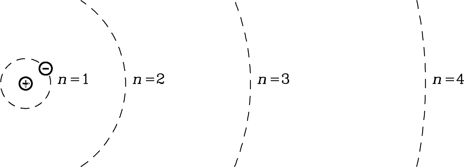
Figure 7.1: The radius of the $n$ th Bohr orbit is proportional to $n^{2}$ , so radio-emitting hydrogen atoms with $n\sim 100$ are $\sim 10^{4}$ times larger than ordinary hydrogen atoms in the $n=1$ ground state.

The electron in a Bohr atom can fall from the level $(n+\Delta n)$ to $n$ , where $\Delta n$ and $n$ are any natural numbers ( $1,~{}2,~{}3,\ldots$ ), by emitting a photon whose energy equals the energy difference $\Delta E$ between the initial and final levels. Such spectral lines are called recombination lines because formerly free electrons recombining with ions quickly cascade to the ground state by emitting such photons. Astronomers label each recombination line using the name of the element, the final level number $n$ , and successive letters in the Greek alphabet to denote the level change $\Delta n$ : $\alpha$ for $\Delta n=1$ , $\beta$ for $\Delta n=2$ , $\gamma$ for $\Delta n=3$ , etc. For example, the recombination line produced by the transition between the $n=92$ and $n=91$ levels of a hydrogen atom is called the H91 $\alpha$ line.

The total electronic energy $E_{n}$ is the sum of the kinetic ( $T$ ) and potential ( $V$ ) energies of the electron in the $n$ th circular orbit:

E_{n}=T+V=-T=V/2=-\frac{e^{2}}{2a_{n}}=-e^{2}\biggl{(}\frac{m_{\mathrm{e}}e^{2% }}{2n^{2}\hbar^{2}}\biggr{)}=-\biggl{(}\frac{m_{\mathrm{e}}e^{4}}{2\hbar^{2}}% \biggr{)}\frac{1}{n^{2}}.

(7.7)

The electronic energy change $\Delta E$ going from level $(n+\Delta n)$ to level $n$ is equal to the energy $h\nu$ of the emitted photon:

\Delta E=\frac{m_{\mathrm{e}}e^{4}}{2\hbar^{2}}\biggl{[}\frac{1}{n^{2}}-\frac{% 1}{(n+\Delta n)^{2}}\biggr{]}=h\nu,

(7.8)

so the photon frequency is

\nu=\biggl{(}\frac{2\pi^{2}m_{\mathrm{e}}e^{4}}{h^{3}c}\biggr{)}c\biggl{[}% \frac{1}{n^{2}}-\frac{1}{(n+\Delta n)^{2}}\biggr{]}.

(7.9)

The factor in large parentheses is called the Rydberg constant $R_{\infty}$ , where the subscript refers to the limit of infinite nuclear mass $M$ :

R_{\infty}\equiv\biggl{(}\frac{2\pi^{2}m_{\mathrm{e}}e^{4}}{h^{3}c}\biggr{)}=1% .09737312\ldots\times 10^{5}\mathrm{~{}cm}^{-1}.

(7.10)

The dimensions of $R_{\infty}$ are length ${}^{-1}$ , and the product $R_{\infty}c$ is the Rydberg frequency:

R_{\infty}c=3.28984\ldots\times 10^{15}\mathrm{~{}Hz}.

(7.11)

Allowing for the relatively large but finite nuclear mass $M\gg m_{\mathrm{e}}$ and repeating the analysis above in the atomic center-of-mass frame yields the same frequency formula with $R_{\infty}$ replaced by $R_{M}$ :

\boxed{\nu=R_{M}c\biggl{[}\frac{1}{n^{2}}-\frac{1}{(n+\Delta n)^{2}}\biggr{]},% \qquad\mathrm{where}\qquad R_{M}\equiv R_{\infty}\biggl{(}1+\frac{m_{\mathrm{e% }}}{M}\biggr{)}^{-1},}

(7.12)

The hydrogen nucleus is a single proton of mass $m_{\mathrm{p}}\approx 1836.1m_{\mathrm{e}}$ so $M(\mathrm{H})\approx 1836.1m_{\mathrm{e}}$ and $R_{M}c$ for a hydrogen atom is

R_{M}c=3.28984\times 10^{15}\,\mathrm{Hz}\biggl{(}1+\frac{1}{1836.1}\biggr{)}^% {-1}=3.28805\times 10^{15}\,\mathrm{Hz}.

Thus the frequency of the photon produced by the H109 $\alpha$ transition ( $n+\Delta n=110$ to $n=109$ ) is

\nu(\mathrm{H}109\alpha)=3.28805\times 10^{15}\,\mathrm{Hz}\biggl{(}\frac{1}{1% 09^{2}}-\frac{1}{110^{2}}\biggr{)}\approx 5.0089\times 10^{9}\,\mathrm{Hz}.

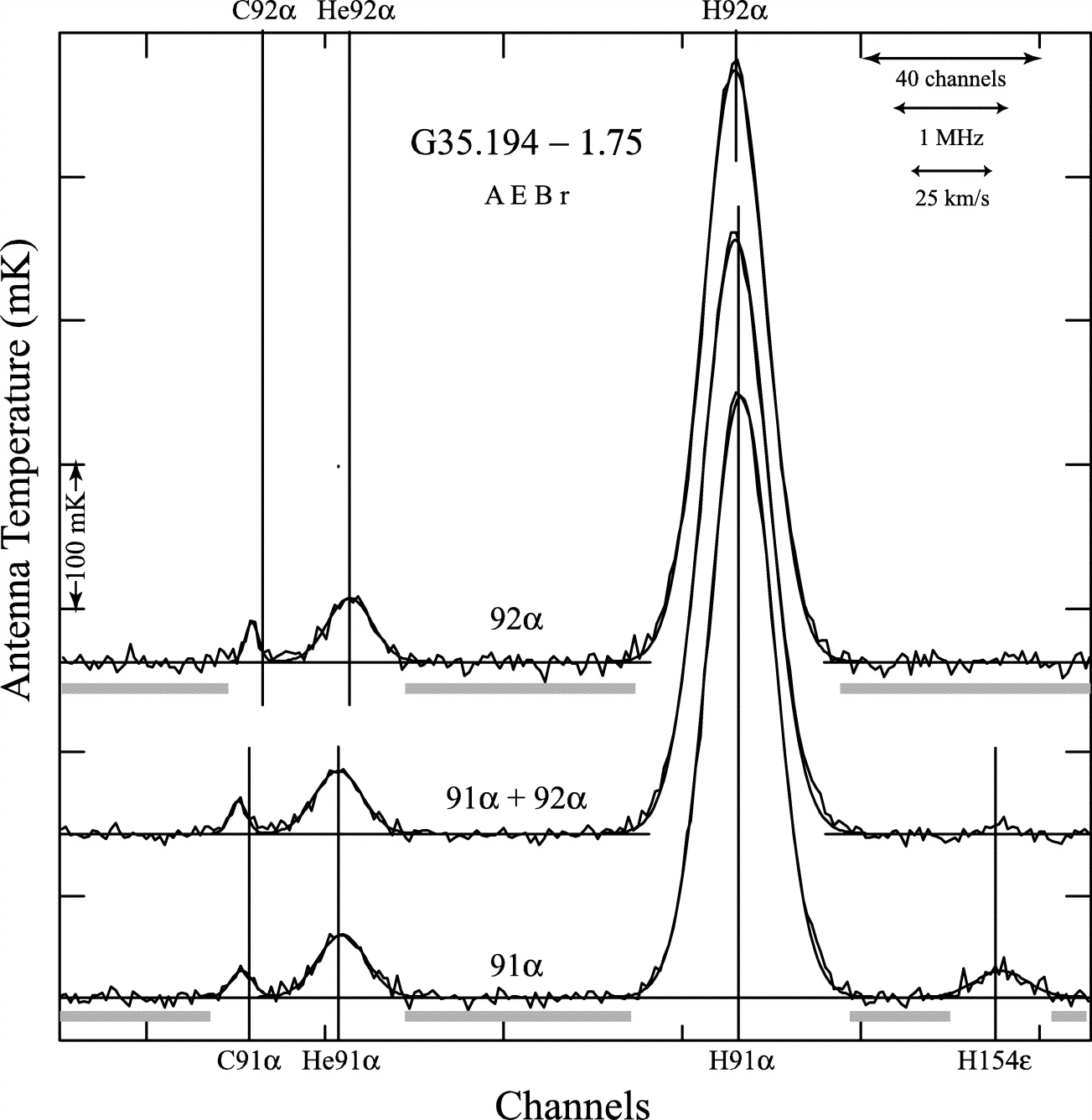
The mass of a neutron is about equal to the mass of a proton, so the ${}^{4}$ He nucleus consisting of two protons and two neutrons has mass $M(^{4}\mathrm{He})\approx 4M(\mathrm{H})$ , the isotope of carbon with six protons and six neutrons has $M(^{12}\mathrm{C})\approx 12M(\mathrm{H})$ , and so on. Electrons recombining onto singly ionized atoms with any number $N_{\mathrm{p}}$ of protons and $(N_{\mathrm{p}}-1)$ electrons orbit in the potential produced by a net charge of one proton, so the recombination lines of heavier atoms are very similar to those of hydrogen, but at the slightly higher frequencies (Figure 7.2) given by Equation 7.12. For example, the primordial abundance of the rare helium isotope ${}^{3}$ He is important because it depends on the photon/baryon ratio in the early universe. The abundance of ${}^{3}$ He in Galactic Hii regions has been measured via radio recombination-line emission and indicates that baryons account for only a few percent of the critical density needed to close the universe.

Figure 7.2: Observed recombination-line spectra from the 91 $\alpha$ and 92 $\alpha$ transitions of hydrogen, helium, and carbon observed in an Hii region [85].

The strongest radio recombination lines are produced by transitions with $\Delta n\ll n$ , so the approximation

\biggl{[}\frac{1}{n^{2}}-\frac{1}{(n+\Delta n)^{2}}\biggr{]}\approx\frac{(n+% \Delta n)^{2}-n^{2}}{n^{2}(n+\Delta n)^{2}}=\frac{n^{2}+2n\Delta n+(\Delta n)^% {2}-n^{2}}{n^{2}[n^{2}+2n\Delta n+(\Delta n)^{2}]}\approx\frac{2n\Delta n}{n^{% 4}}=\frac{2\Delta n}{n^{3}}

(7.13)

yields simpler (but not extremely accurate) approximations for radio recombination line frequencies

\nu\approx\frac{2(R_{M}c)\Delta n}{n^{3}},

(7.14)

and for the frequency separation $\Delta\nu=\nu(n)-\nu(n+1)$ between adjacent lines

\boxed{\frac{\Delta\nu}{\nu}\approx\frac{3}{n}.}

(7.15)

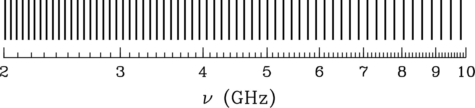
Adjacent high- $n$ (low- $\nu$ ) radio recombination lines have such small fractional frequency separations (Figure 7.3) that two or more transitions can often be observed simultaneously and averaged, to reduce the observing time needed to reach a given signal-to-noise ratio.

Figure 7.3: The $\Delta n=1$ radio recombination lines of singly ionized atoms, shown here as vertical bars, are closely spaced in frequency.

The H109 $\alpha$ line was first detected by P. Mezger in 1965, despite (incorrect) theoretical predictions that pressure broadening would smear out the lines in frequency and make them undetectable. It is true that atomic collisions in the interstellar medium significantly disturb the energy levels of large atoms, but this disturbance is about the same for adjacent energy levels, so the differential disturbance that alters the line frequency is actually much smaller. His advice: “Don’t abandon an observation just because you have been told that it will fail.”

7.2.2 Recombination Line Strengths

The spontaneous emission rate is the average rate at which an isolated atom emits photons. Rigorous quantum-mechanical calculations of spontaneous emission rates are complicated, but a fairly good classical approximation can be derived by noting that radio photons are emitted by atoms with $n\gg 1$ and invoking the correspondence principle, Bohr’s hypothesis that systems with large quantum numbers behave almost classically. The time-averaged radiated power $\langle P\rangle$ for classical transitions is given by Larmor’s formula (Equation 2.143) for an electric dipole with dipole moment $ea_{n}$ :

\langle P\rangle=\frac{2e^{2}}{3c^{3}}(\omega^{2}a_{n})^{2}\langle\cos^{2}(% \omega t)\rangle=\frac{2e^{2}}{3c^{3}}(2\pi\nu)^{4}\frac{a_{n}^{2}}{2}.

(7.16)

The photon emission rate (s ${}^{-1}$ ) equals the average power emitted by one atom divided by the energy of each photon. The spontaneous emission rate for transitions from level $n$ to level $(n-1)$ is denoted by $A_{n,n-1}$ :

A_{n,n-1}=\frac{\langle P\rangle}{h\nu},

(7.17)

where

\nu\approx\frac{2R_{\infty}c\Delta n}{n^{3}}

(7.18)

in the limit $\Delta n\ll n$ (Equation 7.14). In that limit, $A_{n+1,n}\approx A_{n,n-1}$ also.

The atomic radius (Equation 7.6) is

a_{n}\approx\frac{n^{2}h^{2}}{4\pi^{2}m_{\mathrm{e}}e^{2}},

(7.19)

$\displaystyle A_{n+1,n}$	$\displaystyle\approx\frac{\langle P\rangle}{h\nu}\approx\frac{2e^{2}}{3c^{3}}% \biggl{(}\frac{16\pi^{4}\nu^{3}}{h}\biggr{)}\frac{a_{n}^{2}}{2}$	(7.20)
	$\displaystyle\approx\frac{16\pi^{4}}{3}\frac{e^{2}}{c^{3}h}\biggl{(}\frac{2R_{% \infty}c}{n^{3}}\biggr{)}^{3}\biggl{(}\frac{n^{2}h^{2}}{4\pi^{2}m_{\mathrm{e}}% e^{2}}\biggr{)}^{2}$	(7.21)
	$\displaystyle\approx\frac{16\pi^{4}}{3}\frac{e^{2}}{c^{3}h}\biggl{(}\frac{4\pi% ^{2}m_{\mathrm{e}}e^{4}}{h^{3}}\biggr{)}^{3}\biggl{(}\frac{h^{2}}{4\pi^{2}m_{% \mathrm{e}}e^{2}}\biggr{)}^{2}\frac{1}{n^{5}},$	(7.22)

\boxed{A_{n+1,n}\approx\biggl{(}\frac{64\pi^{6}m_{\mathrm{e}}e^{10}}{3c^{3}h^{% 6}}\biggr{)}\frac{1}{n^{5}}.}

(7.23)

Evaluating the constants yields the spontaneous emission rate of hydrogen atoms:

A_{n+1,n}\approx\biggl{[}\frac{64\pi^{6}\cdot 9.11\times 10^{-28}\mathrm{~{}g}% \cdot(4.8\times 10^{-10}\mathrm{~{}statcoul})^{10}}{3\cdot(3\times 10^{10}% \mathrm{~{}cm~{}s}^{-1})^{3}\cdot(6.63\times 10^{-27}\mathrm{~{}erg~{}s})^{6}}% \biggr{]}\frac{1}{n^{5}},

(7.24)

\boxed{A_{n+1,n}\approx 5.3\times 10^{9}\biggl{(}\frac{1}{n^{5}}\biggr{)}% \mathrm{~{}s}^{-1}.}

(7.25)

For example, the 5.0089 GHz H109 $\alpha$ transition rate is $A_{110,109}\approx 0.3\mathrm{~{}s}^{-1}$ .

The associated natural line width or intrinsic line width follows from the uncertainty principle: $\Delta E\Delta t\approx\hbar$ . Substituting $h\Delta\nu$ for $\Delta E$ and $A^{-1}_{\mathrm{n+1},\mathrm{n}}$ for $\Delta t$ for each energy level involved in the transition and summing these two uncertainties yields

\Delta\nu\sim A_{n+1,n}/\pi\sim 0.1\mathrm{~{}Hz}.

(7.26)

Natural broadening is negligibly small at the large $n$ that produce radio-frequency photons. Collisions of the emitting atoms cause collisional broadening, where the amount of collisional broadening is a small fraction of the collision rate when $\Delta n\ll n$ . Except for very large $n$ , collisional broadening is also small and the actual line profile (normalized intensity as a function of frequency) is primarily determined by Doppler shifts reflecting the radial velocities $v_{r}$ of the emitting atoms. The sign convention is $v_{r}>0$ for sources moving away from the observer. Radial velocities may be microscopic (from the thermal motions of individual atoms) or macroscopic (from large-scale turbulence, flows, or rotation). In the nonrelativistic limit $v_{r}\ll c$ , the Doppler equation (Equation 5.142) relating the observed frequency $\nu$ to the line rest frequency $\nu_{0}$ reduces to

\nu\approx\nu_{0}\biggl{(}1-\frac{v_{r}}{c}\biggr{)},

(7.27)

so nonrelativistic radial velocities can be estimated from

v_{r}\approx\frac{c\,(\nu_{0}-\nu)}{\nu_{0}}.

(7.28)

The thermal component of the line profile from a recombination-line source in LTE is determined by the Maxwellian speed distribution (Equation B.49) of atoms with mass $M$ and temperature $T$ . The speed in any one coordinate of an isotropic distribution is $3^{-1/2}$ of the total speed in three dimensions, so the Gaussian

f(v_{r})=\biggl{(}\frac{M}{2\pi kT}\biggr{)}^{1/2}\exp\biggl{(}-\frac{Mv_{r}^{% 2}}{2kT}\biggr{)}

(7.29)

is the normalized ( $\int f(v_{r})\,dv_{r}=1$ ) radial velocity distribution. The normalized line profile (Figure 7.4) $\phi(\nu)$ for thermal emission is

	$\displaystyle\|\phi(\nu)d\nu\|$	$\displaystyle=f(v_{r})dv_{r},$		(7.30)
	$\displaystyle\phi(\nu)$	$\displaystyle=\biggl{(}\frac{M}{2\pi kT}\biggr{)}^{1/2}\exp\biggl{[}-\frac{M}{% 2kT}\frac{c^{2}(\nu-\nu_{0})^{2}}{\nu_{0}^{2}}\biggr{]}\bigg{\|}\frac{dv_{r}}{d% \nu}\bigg{\|},$		(7.31)

\boxed{\phi(\nu)=\frac{c}{\nu_{0}}\biggl{(}\frac{M}{2\pi kT}\biggr{)}^{1/2}% \exp\biggl{[}-\frac{Mc^{2}}{2kT}\frac{(\nu-\nu_{0})^{2}}{\nu_{0}^{2}}\biggr{]}.}

(7.32)

Figure 7.4: The parameters of the normalized ( $\int\phi(\nu)\,d\nu=1$ ) line profile $\phi(\nu)$ are the center frequency $\nu_{0}$ , the FWHM line width $\Delta\nu$ , and the profile height $\phi(\nu_{0})$ at the center frequency.

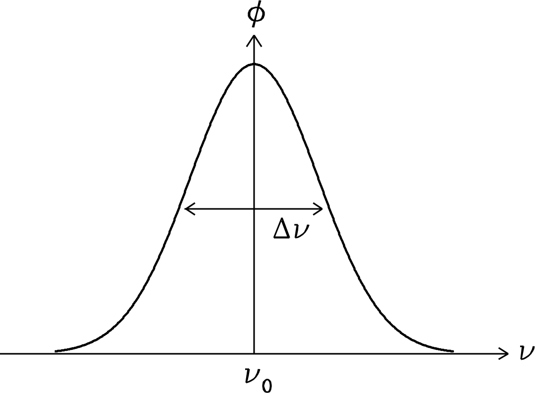
This is a Gaussian line profile. Its full width between half-maximum points (FWHM) $\Delta\nu$ is the solution of

	$\displaystyle\exp\biggl{[}-\frac{Mc^{2}}{2kT}\frac{(\Delta\nu/2)^{2}}{\nu_{0}^% {2}}\biggr{]}=\frac{1}{2},$		(7.33)
	$\displaystyle\frac{Mc^{2}}{2kT}\frac{\Delta\nu^{2}}{4\nu_{0}^{2}}=\ln 2,$		(7.34)
	$\displaystyle\boxed{\Delta\nu=\biggl{[}\frac{8\ln(2)\,k}{c^{2}}\biggr{]}^{1/2}% \biggl{(}\frac{T}{M}\biggr{)}^{1/2}\nu_{0}.}$		(7.35)

For example, the FWHM of the H109 $\alpha$ line ( $\nu_{0}=5.0089$ GHz) in a quiescent (no macroscopic motions) Hii region with temperature $T\approx 10^{4}$ K is

	$\displaystyle\Delta\nu$	$\displaystyle\approx~{}\biggl{[}\frac{8\ln 2\,\cdot\,1.38\times 10^{-16}% \mathrm{~{}erg~{}K}^{-1}}{(3\times 10^{10}\mathrm{~{}cm~{}s}^{-1})^{2}}\biggr{% ]}^{1/2}\biggl{(}\frac{10^{4}\mathrm{~{}K}}{1836\cdot 9.11\times 10^{-28}% \mathrm{~{}g}}\biggr{)}^{1/2}$
		$\displaystyle\quad\times 5.0089\times 10^{9}\mathrm{~{}Hz}$
		$\displaystyle\approx 3.6\times 10^{5}\mathrm{~{}Hz}.$

Notice that the thermal line width $\Delta\nu$ is much larger than the natural line width $A_{110,109}\approx 0.3$ Hz.

Normalization (requiring $\int\phi(\nu)d\nu=1$ ) implies that the value of $\phi$ at the line center ( $\nu=\nu_{0}$ ) is

\phi(\nu_{0})=\frac{c}{\nu_{0}}\biggl{(}\frac{M}{2\pi kT}\biggr{)}^{1/2}=\frac% {c}{\Delta\nu}\biggl{(}\frac{8\ln 2\,kT}{Mc^{2}}\frac{M}{2\pi kT}\biggr{)}^{1/% 2},

(7.36)

\boxed{\phi(\nu_{0})=\biggl{(}\frac{\ln 2}{\pi}\biggr{)}^{1/2}\frac{2}{\Delta% \nu}.}

(7.37)

For a given integrated (over frequency) line strength, the line strength per unit frequency at any one frequency (e.g., at $\nu_{0}$ ) is inversely proportional to the line width $\Delta\nu$ . Integrated line strengths are frequently specified in the astronomically convenient units of $\mathrm{Jy~{}km~{}s}^{-1}$ , where $1\mathrm{~{}km~{}s}^{-1}\approx\nu_{0}/3.00\times 10^{5}$ .

7.3 Line Radiative Transfer

7.3.1 Einstein Coefficients

The spontaneous emission coefficient $A_{\mathrm{UL}}$ is the average photon emission rate (s ${}^{-1}$ ) for an “undisturbed” atom or molecule transitioning from an upper (U) to a lower (L) energy state. The spectral-line radiative transfer problem also involves the absorption coefficient $B_{\mathrm{LU}}$ and the stimulated emission coefficient $B_{\mathrm{UL}}$ (Figure 7.5). Einstein showed that both the absorption and stimulated emission coefficients can be calculated from the spontaneous emission coefficient.

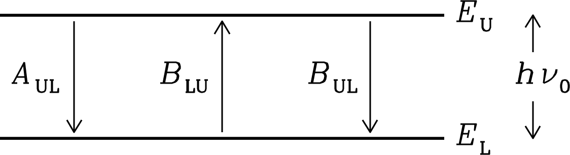
Figure 7.5: The three Einstein coefficients for a two-level system: $A_{\mathrm{UL}}$ for spontaneous emission, $B_{\mathrm{LU}}$ for absorption, and $B_{\mathrm{UL}}$ for stimulated emission.

Consider any two energy levels $E_{\mathrm{U}}$ and $E_{\mathrm{L}}$ of a quantum system such as a single atom or molecule. The photon emitted or absorbed during a transition between the upper and lower states will have energy

E=E_{\mathrm{U}}-E_{\mathrm{L}}

(7.38)

and contribute to a spectral line with rest frequency $\nu_{0}=E/h$ . The energy levels actually have small but finite widths, so the spectral line has some narrow line profile $\phi(\nu)$ centered on $\nu=\nu_{0}$ and conventionally normalized such that $\int_{0}^{\infty}\phi(\nu)\,d\nu=1$ . A system in the lower energy state may absorb a photon of frequency $\nu\approx\nu_{0}$ and transition to the upper state. The rate (s ${}^{-1}$ ) for this process is proportional to the profile-weighted mean radiation energy density

\bar{u}\equiv\int_{0}^{\infty}u_{\nu}(\nu)\,\phi(\nu)\,d\nu

(7.39)

of the surrounding radiation field, so the Einstein absorption coefficient $B_{\mathrm{LU}}$ is defined to make the product

\boxed{B_{\mathrm{LU}}\bar{u}}

(7.40)

equal the average rate (s ${}^{-1}$ ) at which photons are absorbed by a single atomic or molecular system in its lower energy state.

Einstein realized that there must be a third process in addition to spontaneous emission and absorption. It is stimulated emission, in which a photon of energy $E=h\nu_{0}$ stimulates the system in the upper energy state to emit a second photon with the same energy and direction. The rate for this process is also proportional to $\bar{u}$ , so by analogy with Equation 7.40, the Einstein stimulated-emission coefficient $B_{\mathrm{UL}}$ is defined to make the product

\boxed{B_{\mathrm{UL}}\bar{u}}

(7.41)

equal the average rate (s ${}^{-1}$ ) of stimulated photon emission by a single quantum system in its upper energy state. Beware that some authors use $\bar{I}$ instead of $\bar{u}$ in Equation 7.41 to define a stimulated emission coefficient that is $4\pi/c$ times the $B_{\mathrm{UL}}$ given by Equation 7.41 [98].

Stimulated emission is sometimes called negative absorption. Negative absorption is not familiar in everyday life because it is much weaker in room-temperature objects at visible wavelengths, where $h\nu/(kT)\gg 1$ , but negative absorption competes effectively with ordinary absorption at radio wavelengths where $h\nu/(kT)\ll 1$ .

Consider a macroscopic collection of many atoms or molecules in full thermodynamic equilibrium (TE) with the surrounding radiation field. TE is a stationary state. If there are $(n_{\mathrm{U}},\,n_{\mathrm{L}})$ atoms or molecules per unit volume in the (upper, lower) energy states, then the average rate of photon creation by both spontaneous emission and stimulated emission must balance the average rate of photon destruction by absorption:

\boxed{n_{\mathrm{U}}A_{\mathrm{UL}}+n_{\mathrm{U}}B_{\mathrm{UL}}\bar{u}=n_{% \mathrm{L}}B_{\mathrm{LU}}\bar{u}.}

(7.42)

In TE, the ratio of $n_{\mathrm{U}}$ to $n_{\mathrm{L}}$ is fixed by the Boltzmann equation

\frac{n_{\mathrm{U}}}{n_{\mathrm{L}}}=\frac{g_{\mathrm{U}}}{g_{\mathrm{L}}}\,% \exp\biggl{[}-\frac{(E_{\mathrm{U}}-E_{\mathrm{L}})}{kT}\biggr{]}=\frac{g_{% \mathrm{U}}}{g_{\mathrm{L}}}\,\exp\biggl{(}-\frac{h\nu_{0}}{kT}\biggr{)},

(7.43)

where $g_{\mathrm{U}}$ and $g_{\mathrm{L}}$ are the numbers of distinct physical states having energies $E_{\mathrm{U}}$ and $E_{\mathrm{L}}$ , respectively. The quantities $g_{\mathrm{U}}$ and $g_{\mathrm{L}}$ are called the statistical weights of those energy states. Examples of statistical weights include the following:

1.

Hydrogen atoms have $g_{n}=2n^{2}$ , where ${n}=1,~{}2,~{}3,\,\ldots$ is the principal quantum number. The number $2n^{2}$ is the product of the 2 electron spin states and $n^{2}$ orbital angular momentum states in the $n$ th electronic energy level.
2.

Rotating linear molecules (e.g., carbon monoxide, CO) have $g=2J+1$ , where $J=0,~{}1,~{}2,\,\ldots$ is the angular-momentum quantum number. For each $J$ , there are $2J+1$ possible values of the $z$ -component of the angular momentum: $J_{z}=-J,-(J-1),\ldots,-1,0,1,\ldots,(J-1),J$ .
3.

Hydrogen atoms have two hyperfine energy levels whose difference yields the $\lambda=21$ cm ( $\nu_{0}=1420.406\ldots$ MHz) Hi line: $g_{\mathrm{U}}=3$ and $g_{\mathrm{L}}=1$ .

Solving Equation 7.42 for the profile-weighted mean energy density $\bar{u}$ of blackbody radiation connects the properties of the quantum system (atom or molecule) to the radiation, just as Kirchhoff’s law (Equation 2.30) did for continuum radiation:

\bar{u}=\frac{n_{\mathrm{U}}A_{\mathrm{UL}}}{n_{\mathrm{L}}B_{\mathrm{LU}}-n_{% \mathrm{U}}B_{\mathrm{UL}}}=\frac{A_{\mathrm{UL}}}{(n_{\mathrm{L}}/n_{\mathrm{% U}})B_{\mathrm{LU}}-B_{\mathrm{UL}}}.

(7.44)

For full TE at temperature $T$ , Equations 7.43 and 7.44 imply

\bar{u}=A_{\mathrm{UL}}\biggl{[}\frac{g_{\mathrm{L}}}{g_{\mathrm{U}}}\exp% \biggl{(}\frac{h\nu_{0}}{kT}\biggr{)}B_{\mathrm{LU}}-B_{\mathrm{UL}}\biggr{]}^% {-1}

(7.45)

for matter and Equation 2.92 implies

\bar{u}=\frac{4\pi}{c}\int_{0}^{\infty}B_{\nu}(T)\,\phi(\nu)d\nu

(7.46)

for radiation. Inserting the Planck radiation law (Equation 2.86) for $B_{\nu}(T)$ near $\nu=\nu_{0}$ gives

\bar{u}\approx\frac{4\pi}{c}\frac{2h\nu_{0}^{3}}{c^{2}}\biggl{[}\exp\biggl{(}% \frac{h\nu_{0}}{kT}\biggr{)}-1\biggr{]}^{-1}.

(7.47)

Equations 7.45 and 7.47 for $\bar{u}$ must agree:

A_{\mathrm{UL}}\biggl{[}\frac{g_{\mathrm{L}}}{g_{\mathrm{U}}}\exp\biggl{(}% \frac{h\nu_{0}}{kT}\biggr{)}B_{\mathrm{LU}}-B_{\mathrm{UL}}\biggr{]}^{-1}=% \frac{4\pi}{c}\frac{2h\nu_{0}^{3}}{c^{2}}\biggl{[}\exp\biggl{(}\frac{h\nu_{0}}% {kT}\biggr{)}-1\biggr{]}^{-1}

(7.48)

for all temperatures $T$ , so the equation

\frac{A_{\mathrm{UL}}}{B_{\mathrm{UL}}}\biggl{[}\frac{g_{\mathrm{L}}}{g_{% \mathrm{U}}}\frac{B_{\mathrm{LU}}}{B_{\mathrm{UL}}}\exp\biggl{(}\frac{h\nu_{0}% }{kT}\biggr{)}-1\biggr{]}^{-1}=\frac{8\pi h\nu_{0}^{3}}{c^{3}}\biggl{[}\exp% \biggl{(}\frac{h\nu_{0}}{kT}\biggr{)}-1\biggr{]}^{-1}

(7.49)

implies both

\boxed{\frac{g_{\mathrm{L}}}{g_{\mathrm{U}}}\frac{B_{\mathrm{LU}}}{B_{\mathrm{% UL}}}=1}

(7.50)

and

\boxed{\frac{A_{\mathrm{UL}}}{B_{\mathrm{UL}}}=\frac{8\pi h\nu_{0}^{3}}{c^{3}}.}

(7.51)

Equations 7.50 and 7.51 are called the equations of detailed balance. The two equations relate the three quantities $A_{\mathrm{UL}}$ , $B_{\mathrm{LU}}$ , and $B_{\mathrm{UL}}$ , so all three can be computed if only one (e.g., the spontaneous emission coefficient $A_{\mathrm{UL}}$ ) is known. Equations 7.50 and 7.51 also prove that $B_{\mathrm{UL}}$ cannot be zero; that is, stimulated emission must occur.

Note that these Equations 7.50 and 7.51 are valid for any microscopic physical system because they relate the coefficients $A_{\mathrm{UL}}$ , $B_{\mathrm{UL}}$ , and $B_{\mathrm{LU}}$ , characteristic of individual atoms or molecules for which the macroscopic statistical concepts of TE or LTE are meaningless. Although TE was assumed for their derivation, the dependences on temperature $T$ and frequency $\nu$ dropped out for a line at a single frequency $\nu_{0}$ . Thus Equations 7.50 and 7.51 also apply to all macroscopic systems, whether or not they are in TE or even LTE. (Recall the derivation of Kirchhoff’s law $j_{\nu}(T)/\kappa(T)=B_{\nu}(T)$ (Equation 2.30), which also made use of full TE but also relates the emission and absorption coefficients of any matter in LTE at temperature $T$ , independent of the actual ambient radiation field.)

7.3.2 Radiative Transfer and Detailed Balance

The two Equations 7.50 and 7.51 for detailed balance relate the three Einstein coefficients and allow the spectral-line radiative transfer problem to be solved in terms of the spontaneous emission coefficient $A_{\mathrm{UL}}$ alone. The radiative transfer equation (2.27) is

\frac{dI_{\nu}}{ds}=-\kappa I_{\nu}+j_{\nu},

(7.52)

where $I_{\nu}$ is the specific intensity, $\kappa$ is the net fraction of photons absorbed (the difference between ordinary absorption and negative absorption) per unit length, and $j_{\nu}$ is the volume emission coefficient.

The ordinary opacity coefficient is the fraction of spectral brightness removed per unit length by absorption from the lower level to the upper level. At frequencies near the line center frequency $\nu_{0}$ , the photon energy is $h\nu_{0}$ , the number of absorbers per unit volume is $n_{\mathrm{L}}$ , the number of absorptions per unit area per unit time is $n_{\mathrm{L}}B_{\mathrm{LU}}$ , the fraction of photons absorbed per unit area per unit length is $n_{\mathrm{L}}B_{\mathrm{LU}}/c$ , and the photon energy loss per unit length at frequency $\nu$ is

\frac{dI_{\nu}}{ds}=-\kappa I_{\nu}=-\biggl{(}\frac{h\nu_{0}}{c}\biggr{)}n_{% \mathrm{L}}B_{\mathrm{LU}}\phi(\nu)I_{\nu}.

(7.53)

Stimulated emission is best treated as negative absorption because, like ordinary absorption and unlike spontaneous emission, its strength is proportional to $I_{\nu}$ . The derivation of Equation 7.53 can be repeated to give

\frac{dI_{\nu}}{ds}=-\kappa I_{\nu}=\biggl{(}\frac{h\nu_{0}}{c}\biggr{)}n_{% \mathrm{U}}B_{\mathrm{UL}}\phi(\nu)I_{\nu}.

(7.54)

Adding Equations 7.53 and 7.54 yields the net absorption coefficient

\kappa=\biggl{(}\frac{h\nu_{0}}{c}\biggr{)}(n_{\mathrm{L}}B_{\mathrm{LU}}-n_{% \mathrm{U}}B_{\mathrm{UL}})\phi(\nu).

(7.55)

The spontaneous emission coefficient is the spectral brightness (power per unit frequency per steradian) added per unit volume by spontaneous transitions from the upper to lower energy levels. As above, the line photon energy is approximately $h\nu_{0}$ , the number density in the upper energy level is $n_{\mathrm{U}}$ , and the photon emission rate per unit volume is $n_{\mathrm{U}}A_{\mathrm{UL}}$ . These photons are emitted isotropically over $4\pi\mathrm{~{}sr}$ , so

\frac{dI_{\nu}}{ds}=j_{\nu}=\biggl{(}\frac{h\nu_{0}}{4\pi}\biggr{)}n_{\mathrm{% U}}A_{\mathrm{UL}}\phi(\nu).

(7.56)

Inserting the net absorption coefficient (Equation 7.55) and the spontaneous emission coefficient (Equation 7.56) into Equation 7.52 specifies the full spectral-line equation of radiative transfer:

\boxed{\frac{dI_{\nu}}{ds}=-\biggl{(}\frac{h\nu_{0}}{c}\biggr{)}(n_{\mathrm{L}% }B_{\mathrm{LU}}-n_{\mathrm{U}}B_{\mathrm{UL}})\phi(\nu)I_{\nu}+\biggl{(}\frac% {h\nu_{0}}{4\pi}\biggr{)}n_{\mathrm{U}}A_{\mathrm{UL}}\phi(\nu).}

(7.57)

Equation 7.50 can be used to eliminate the stimulated emission coefficient $B_{\mathrm{UL}}$ in Equation 7.55 and yield

\kappa=\biggl{(}\frac{h\nu_{0}}{c}\biggr{)}n_{\mathrm{L}}B_{\mathrm{LU}}\biggl% {(}1-\frac{n_{\mathrm{U}}}{n_{\mathrm{L}}}\frac{g_{\mathrm{L}}}{g_{\mathrm{U}}% }\biggr{)}\phi(\nu).

(7.58)

The ratio of the emission coefficient to the net absorption coefficient is

\frac{j_{\nu}}{\kappa}=\frac{cn_{\mathrm{U}}A_{\mathrm{UL}}}{4\pi n_{\mathrm{L% }}B_{\mathrm{LU}}}\biggl{(}1-\frac{n_{\mathrm{U}}}{n_{\mathrm{L}}}\frac{g_{% \mathrm{L}}}{g_{\mathrm{U}}}\biggr{)}^{-1}.

(7.59)

Equation 7.50 can be used to eliminate $A_{\mathrm{UL}}$ from this ratio also:

\frac{j_{\nu}}{\kappa}=\frac{n_{\mathrm{U}}(8\pi h\nu_{0}^{3}/c^{2})B_{\mathrm% {UL}}}{4\pi n_{\mathrm{L}}B_{\mathrm{LU}}}\biggl{(}1-\frac{n_{\mathrm{U}}}{n_{% \mathrm{L}}}\frac{g_{\mathrm{L}}}{g_{\mathrm{U}}}\biggr{)}^{-1}=\frac{2h\nu_{0% }^{3}}{c^{2}}\frac{B_{\mathrm{UL}}}{B_{\mathrm{LU}}}\biggl{(}\frac{n_{\mathrm{% L}}}{n_{\mathrm{U}}}-\frac{g_{\mathrm{L}}}{g_{\mathrm{U}}}\biggr{)}^{-1}.

(7.60)

Finally, Equation 7.51 can be used to eliminate both $B_{\mathrm{UL}}$ and $B_{\mathrm{LU}}$ :

\frac{j_{\nu}}{\kappa}=\frac{2h\nu_{0}^{3}}{c^{2}}\biggl{(}\frac{g_{\mathrm{U}% }}{g_{\mathrm{L}}}\frac{n_{\mathrm{L}}}{n_{\mathrm{U}}}-1\biggr{)}^{-1}.

(7.61)

In LTE, Kirchhoff’s law independently implies

\frac{j_{\nu}}{\kappa}=B_{\nu}(T)=\frac{2h\nu^{3}}{c^{2}}\biggl{[}\exp\biggl{(% }\frac{h\nu}{kT}\biggr{)}-1\biggr{]}^{-1},

(7.62)

\frac{g_{\mathrm{U}}}{g_{\mathrm{L}}}\frac{n_{\mathrm{L}}}{n_{\mathrm{U}}}=% \exp\biggl{(}\frac{h\nu_{0}}{kT}\biggr{)},

(7.63)

recovering the Boltzmann equation (Equation 7.43) for LTE (not just for full TE):

\boxed{\frac{n_{\mathrm{U}}}{n_{\mathrm{L}}}=\frac{g_{\mathrm{U}}}{g_{\mathrm{% L}}}\exp\biggl{(}-\frac{h\nu_{0}}{kT}\biggr{)}.}

(7.64)

Equation 7.58 and the assumption of LTE allows the substitution of

B_{\mathrm{LU}}=\frac{g_{\mathrm{U}}}{g_{\mathrm{L}}}B_{\mathrm{UL}}=\frac{g_{% \mathrm{U}}}{g_{\mathrm{L}}}\frac{A_{\mathrm{UL}}c^{3}}{8\pi h\nu_{0}^{3}}

(7.65)

and

\frac{n_{\mathrm{U}}g_{\mathrm{L}}}{n_{\mathrm{L}}g_{\mathrm{U}}}=\exp\biggl{(% }-\frac{h\nu_{0}}{kT}\biggr{)}

(7.66)

to yield the net line opacity coefficient in LTE:

\boxed{\kappa(\nu)=\frac{c^{2}}{8\pi\nu_{0}^{2}}\frac{g_{\mathrm{U}}}{g_{% \mathrm{L}}}n_{\mathrm{L}}A_{\mathrm{UL}}\biggl{[}1-\exp\biggl{(}-\frac{h\nu_{% 0}}{kT}\biggr{)}\biggr{]}\phi(\nu)}

(7.67)

in terms of the spontaneous emission rate $A_{\mathrm{UL}}$ only; the stimulated emission coefficient $B_{\mathrm{UL}}$ and absorption coefficient $B_{\mathrm{LU}}$ have been eliminated.

The quantity

\biggl{[}1-\exp\biggl{(}-\frac{h\nu_{0}}{kT}\biggr{)}\biggr{]}

(7.68)

in Equation 7.67 is the sum of two terms, the first representing ordinary absorption and the second accounting for the negative absorption of stimulated emission. In the Rayleigh–Jeans limit $h\nu_{0}\ll kT$ ,

\biggl{[}1-\exp\biggl{(}-\frac{h\nu_{0}}{kT}\biggr{)}\biggr{]}\approx\frac{h% \nu_{0}}{kT}\ll 1.

(7.69)

Thus stimulated emission nearly cancels pure absorption and significantly reduces the net line opacity at radio frequencies. Because $\kappa\propto T^{-1}$ and $B_{\nu}\propto T$ , the product $\kappa B_{\nu}$ is independent of temperature. The brightness of an optically thin ( $\tau\ll 1$ ) radio emission line is proportional to the column density of emitting gas but can be nearly independent of the gas temperature. Thus the Hi line flux ( $\mathrm{Jy~{}km~{}s}^{-1}$ ) of an optically thin galaxy is proportional to the total mass of neutral hydrogen in the galaxy but says nothing about its temperature.

7.4 Excitation Temperature

Even if a macroscopic two-level system is not in LTE, its excitation temperature $T_{\mathrm{x}}$ can be defined by

\boxed{\frac{n_{\mathrm{U}}}{n_{\mathrm{L}}}\equiv\frac{g_{\mathrm{U}}}{g_{% \mathrm{L}}}\exp\biggl{(}-\frac{h\nu_{0}}{kT_{\mathrm{x}}}\biggr{)}.}

(7.70)

The excitation temperature is not a real temperature; it only measures the ratio of $n_{\mathrm{U}}$ to $n_{\mathrm{L}}$ . In a two-level system, the excitation temperature is determined by a balance between radiative and collisional excitations and de-excitations. If collisions cause $n_{\mathrm{L}}C_{\mathrm{LU}}$ excitations per unit volume per unit time from the lower level to the upper level and $n_{\mathrm{U}}C_{\mathrm{UL}}$ de-excitations per unit volume per unit time from the upper level to the lower level, then Equation 7.42 becomes

\boxed{n_{\mathrm{U}}(A_{\mathrm{UL}}+B_{\mathrm{UL}}\bar{u}+C_{\mathrm{UL}})=% n_{\mathrm{L}}(B_{\mathrm{LU}}\bar{u}+C_{\mathrm{LU}})}

(7.71)

and detailed balance requires

n_{\mathrm{L}}C_{\mathrm{LU}}=n_{\mathrm{U}}C_{\mathrm{UL}}.

(7.72)

Thus

\frac{n_{\mathrm{U}}}{n_{\mathrm{L}}}=\frac{B_{\mathrm{LU}}\bar{u}+C_{\mathrm{% LU}}}{A_{\mathrm{UL}}+B_{\mathrm{UL}}\bar{u}+C_{\mathrm{UL}}}.

(7.73)

Equations 7.47 and 7.51 can be combined to eliminate

B_{\mathrm{UL}}\bar{u}=\frac{c^{3}A_{\mathrm{UL}}}{8\pi h\nu_{0}^{3}}\frac{8% \pi h\nu_{0}^{3}}{c^{3}}\biggl{[}\exp\biggl{(}\frac{h\nu_{0}}{kT_{\mathrm{b}}}% \biggl{)}-1\biggr{]}^{-1}=A_{\mathrm{UL}}\biggl{[}\exp\biggl{(}\frac{h\nu_{0}}% {kT_{\mathrm{b}}}\biggl{)}-1\biggr{]}^{-1},

(7.74)

where $T_{\mathrm{b}}$ is the ambient radiation brightness temperature, in favor of $A_{\mathrm{UL}}$ . Equation 7.50 eliminates

B_{\mathrm{LU}}\bar{u}=B_{\mathrm{UL}}\bar{u}\frac{g_{\mathrm{U}}}{g_{\mathrm{% L}}}=A_{\mathrm{UL}}\frac{g_{\mathrm{U}}}{g_{\mathrm{L}}}\biggl{[}\exp\biggl{(% }\frac{h\nu_{0}}{kT_{\mathrm{b}}}\biggl{)}-1\biggr{]}^{-1}.

(7.75)

Finally, Equations 7.64 and 7.72 allow the replacement

C_{\mathrm{LU}}=\frac{n_{\mathrm{U}}}{n_{\mathrm{L}}}C_{\mathrm{UL}}=\frac{g_{% \mathrm{U}}}{g_{\mathrm{L}}}\exp\biggl{(}-\frac{h\nu_{0}}{kT_{\mathrm{k}}}% \biggr{)}C_{\mathrm{UL}},

(7.76)

where $T_{\mathrm{k}}$ is the kinetic temperature of the gas. The numerator of Equation 7.73 becomes

A_{\mathrm{UL}}\frac{g_{\mathrm{U}}}{g_{\mathrm{L}}}\biggl{[}\exp\biggl{(}% \frac{h\nu_{0}}{kT_{\mathrm{b}}}\biggl{)}-1\biggr{]}^{-1}+\frac{g_{\mathrm{U}}% }{g_{\mathrm{L}}}\exp\biggl{(}-\frac{h\nu_{0}}{kT_{\mathrm{k}}}\biggr{)}C_{% \mathrm{UL}}

(7.77)

and the denominator is

A_{\mathrm{UL}}+A_{\mathrm{UL}}\biggl{[}\exp\biggl{(}\frac{h\nu_{0}}{kT_{% \mathrm{b}}}\biggr{)}-1\biggr{]}^{-1}+C_{\mathrm{UL}}.

(7.78)

Thus

	$\displaystyle\frac{n_{\mathrm{U}}g_{\mathrm{L}}}{n_{\mathrm{L}}g_{\mathrm{U}}}$	$\displaystyle=\frac{\displaystyle A_{\mathrm{UL}}+C_{\mathrm{UL}}\exp\biggl{(}% -\frac{h\nu_{0}}{kT_{\mathrm{k}}}\biggr{)}\biggl{[}\exp\biggl{(}\frac{h\nu_{0}% }{kT_{\mathrm{b}}}\biggr{)}-1\biggr{]}}{\displaystyle A_{\mathrm{UL}}\exp% \biggl{(}\frac{h\nu_{0}}{kT_{\mathrm{b}}}\biggr{)}+C_{\mathrm{UL}}\biggl{[}% \exp\biggl{(}\frac{h\nu_{0}}{kT_{\mathrm{b}}}\biggr{)}-1\biggr{]}},$		(7.79)
	$\displaystyle\exp\biggl{(}-\frac{h\nu_{0}}{kT_{\mathrm{x}}}\biggr{)}$	$\displaystyle=\exp\biggl{(}-\frac{h\nu_{0}}{kT_{\mathrm{b}}}\biggr{)}\frac{% \displaystyle A_{\mathrm{UL}}+C_{\mathrm{UL}}\exp\biggl{(}-\frac{h\nu_{0}}{kT_% {\mathrm{k}}}\biggr{)}\biggl{[}\exp\biggl{(}\frac{h\nu_{0}}{kT_{\mathrm{b}}}% \biggr{)}-1\biggr{]}}{\displaystyle A_{\mathrm{UL}}+C_{\mathrm{UL}}\biggl{[}1-% \exp\biggl{(}-\frac{h\nu_{0}}{kT_{\mathrm{b}}}\biggr{)}\biggr{]}}.$		(7.80)

If the spontaneous emission rate is much larger than the collision rate, Equation 7.80 yields $T_{\mathrm{x}}\rightarrow T_{\mathrm{b}}$ ; if the collision rate is much higher than the spontaneous emission rate, $T_{\mathrm{x}}\rightarrow T_{\mathrm{k}}$ . For any $A_{\mathrm{UL}}$ and $C_{\mathrm{UL}}$ , $T_{\mathrm{x}}$ lies between $T_{\mathrm{k}}$ and $T_{\mathrm{b}}$ .

7.5 Masers

If the upper energy level is overpopulated, that is,

\frac{n_{\mathrm{U}}}{n_{\mathrm{L}}}>\frac{g_{\mathrm{U}}}{g_{\mathrm{L}}},

(7.81)

then $T_{\mathrm{x}}$ is actually negative,

\biggl{[}1-\exp\biggl{(}-\frac{h\nu_{0}}{kT_{\mathrm{x}}}\biggr{)}\biggr{]}

(7.82)

is negative, and Equation 7.67 gives a negative net opacity coefficient $\kappa$ . Negative net opacity implies brightness gain instead of loss; the intensity of a background source at frequency $\nu_{0}$ will be amplified. At radio wavelengths this phenomenon is called maser (an acronym for microwave amplification by stimulated emission of radiation) amplification. Astronomical masers are common at radio frequencies because $h\nu\ll kT$ and hence $n_{\mathrm{U}}/n_{\mathrm{L}}\approx g_{\mathrm{U}}/g_{\mathrm{L}}$ even in TE. These sources can have line brightness temperatures as high as $10^{15}$ K, which is much higher than the kinetic temperature of the masing gas. For a clear presentation covering the basics of astronomical masers, written by Reid & Moran, see Verschuur and Kellermann [110, Chapter 6].

Our model for an astronomical maser starts with the radiative transfer equation for a two-level system. Assume for simplicity that $g_{\mathrm{U}}=g_{\mathrm{L}}$ so that Equation 7.50 implies $B_{\mathrm{LU}}=B_{\mathrm{UL}}\equiv B$ and Equation 7.51 implies $A_{\mathrm{UL}}=8\pi h\nu_{0}^{3}B/c^{3}\equiv A$ . Then Equation 7.57 simplifies to

\frac{dI_{\nu}}{ds}=-\biggl{(}\frac{h\nu_{0}}{c}\biggr{)}(n_{\mathrm{L}}-n_{% \mathrm{U}})B\phi(\nu)I_{\nu}+\biggl{(}\frac{h\nu_{0}}{4\pi}\biggr{)}n_{% \mathrm{U}}A\phi(\nu).

(7.83)

Next assume that the line profile $\phi(\nu)$ is Gaussian with FWHM $\Delta\nu$ (Figure 7.4) so that Equation 7.37 applies and make the numerical approximation

\phi(\nu_{0})=\biggl{(}\frac{\ln\,2}{\pi}\biggr{)}^{1/2}\frac{2}{\Delta\nu}=% \frac{0.939\ldots}{\Delta\nu}\approx\frac{1}{\Delta\nu}.

(7.84)

Then at the line center frequency $\nu_{0}$ ,

\frac{dI_{\nu}}{ds}=-\frac{h\nu_{0}(n_{\mathrm{L}}-n_{\mathrm{U}})BI_{\nu}}{c% \Delta\nu}+\frac{h\nu_{0}n_{\mathrm{U}}A}{4\pi\Delta\nu}.

(7.85)

The maser optical depth

\tau=\int\kappa\,ds=\int\frac{dI_{\nu}}{I_{\nu}}=\frac{h\nu_{0}B}{c\Delta\nu}% \int(n_{\mathrm{U}}-n_{\mathrm{L}})ds

(7.86)

is called the maser gain over the path of integration, and the maser amplifies the intensity of background radiation by the factor $\exp(|\tau|)$ . In a laboratory maser, radiation is trapped in a high-Q resonant cavity to create effective path lengths up to $10^{9}$ times the cavity length. In an astronomical maser there is no cavity, so the radiation makes only a single pass and the physical path must be much longer ( $s>10^{13}\mathrm{~{}cm}$ ) for significant gain to occur.

Maser emission quickly depopulates the upper energy level, so masers have to be “pumped” to emit continuously. Typically one or more higher energy levels absorb radiation from a pump source (e.g., infrared continuum from a star or an AGN), and radiative decays preferentially repopulate the upper energy level. This radiative pumping process produces no more than one maser photon per pump photon, so the pump energy required is proportional to the frequency $\nu=E/h$ of the pump photon. If the maser photon emission rate is limited by the pump luminosity, the maser is described as being saturated; if the pump power is more than adequate, the maser is unsaturated.

Strong, compact maser sources are powerful tools for high-resolution imaging and precision astrometry. They are being used to measure accurate trigonometric distances to individual stars in our Galaxy, the size and structure of our Galaxy, black-hole masses in AGNs, and distances to galaxies up to $\sim 150\mathrm{~{}Mpc}$ [89].

The most spectacular example is the circumnuclear 22 GHz $\mathrm{H}_{2}\mathrm{O}$ megamaser disk surrounding the Seyfert nucleus of NGC 4258 [74] and illustrated in Figure 7.6. The observed maser spectrum has hundreds of narrow lines in three groups clustered around the systemic recession velocity $v\approx 450\mathrm{~{}km~{}s}^{-1}$ of NGC 4258 and at velocities further redshifted and blueshifted by the $v_{\mathrm{rot}}\sim 900\mathrm{~{}km~{}s}^{-1}$ rotation velocities in the disk.

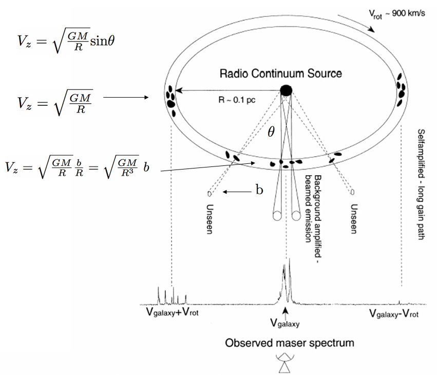
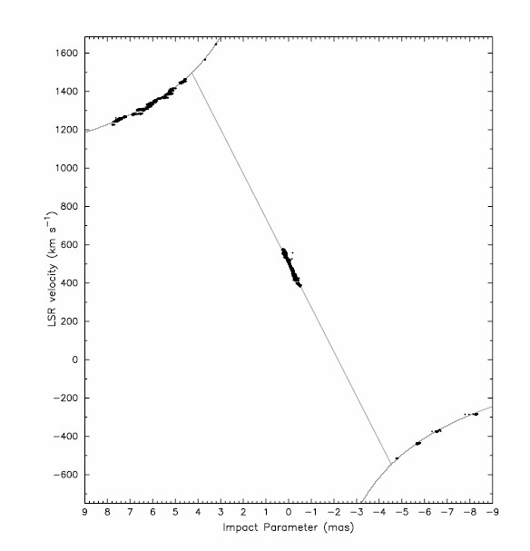
Figure 7.6: A simple ring model illustrating the geometry and kinematics of the edge-on 22 GHz water-maser disk orbiting the nucleus of NGC 4258 [74].

The nearly edge-on maser disk was imaged with high spectral and angular resolution by the VLBA, and its rotation curve is shown in Figure 7.7. The systemic lines are concentrated within a region $<1\mathrm{~{}mas}\approx 0.03\mathrm{~{}pc}$ wide and centered on the line of sight to the supermassive black hole (SMBH) at the center of the disk. Photons from the central radio continuum source are amplified and beamed in our direction, so systemic maser clouds are visible only when they are within a small angle $|\theta|<0.07\mathrm{~{}rad}$ from the line of sight. For a constant $v_{\mathrm{rot}}$ , their $v_{z}=(GM/R^{3})^{1/2}b$ yields the sloped straight line in Figure 7.7. This slope corresponds to the gravitational acceleration $a_{z}=GM/R^{2}$ of the SMBH, and long-term monitoring the velocities of individual systemic-maser lines independently yields $a\approx 8\mathrm{~{}km~{}s}^{-1}\mathrm{~{}yr}^{-1}$ . The redshifted and blueshifted maser clouds are visible only near the tangent points of the disk near $\theta=\pm\pi/2\mathrm{~{}rad}$ , which have the longest gain paths at nearly constant velocities $v_{z}=(GM/R)^{1/2}$ that follow the perfectly Keplerian curves in Figure 7.7. Combining the acceleration, velocity, and angular-size measurements yields a unique solution for both the SMBH mass $M\approx 3.8\times 10^{7}M_{\odot}$ and the distance $D=7.2\pm 0.4\mathrm{~{}Mpc}$ to NGC 4258.

Figure 7.7: The NGC 4258 rotation curve is perfectly Keplerian, indicating that the mass interior to the maser disk is dominated by a single compact object whose density is too high ( $>5\times 10^{12}M_{\odot}\mathrm{~{}pc}^{-3}$ ) for it to be a compact star cluster; it must be an SMBH [74].

7.6 Recombination Line Sources

Astronomical sources of radio recombination lines are often in local thermodynamic equilibrium (LTE). The spontaneous emission rate from atomic physics and the laws of radiative transfer for spectral lines can be combined to model sources in LTE. However, LTE does not apply to all recombination lines, so departures from LTE must be recognized and treated differently.

7.6.1 Radiative Transfer in LTE

Equation 7.67 gives the absorption coefficient at the center frequency $\nu_{0}$ of the $n\rightarrow n+1$ electronic transition of hydrogen in an Hii region in local thermodynamic equilibrium (LTE) at electron temperature $T_{\mathrm{e}}$ :

\kappa(\nu)=\frac{c^{2}}{8\pi\nu^{2}_{0}}\frac{g_{n+1}}{g_{n}}n_{n}A_{n+1,n}% \biggl{[}1-\exp\biggl{(}-\frac{h\nu_{0}}{kT_{\mathrm{e}}}\biggr{)}\biggr{]}% \phi(\nu),

(7.87)

where

	$\displaystyle\nu_{0}$	$\displaystyle=\nu_{n,n+1}\approx\frac{2R_{\infty}c}{n^{3}}=\frac{4\pi^{2}m_{% \mathrm{e}}e^{4}}{h^{3}n^{3}},$		(7.88)
	$\displaystyle g_{n}$	$\displaystyle=2n^{2},$		(7.89)

and $n_{n}$ is the number density of atoms in the $n$ th electronic energy level. At radio frequencies, it can be assumed that $n\gg 1$ , $h\nu_{0}\ll kT_{\mathrm{e}}$ , and $g_{n+1}/g_{n}\approx 1$ . Equation 7.23 gives the spontaneous emission rate

A_{n+1,n}\approx\frac{64\pi^{6}m_{\mathrm{e}}e^{10}}{3c^{3}h^{6}n^{5}}

(7.90)

and Equation 7.37 parameterizes the normalized line profile

\phi(\nu_{0})\approx\biggl{(}\frac{\ln 2}{\pi}\biggr{)}^{1/2}\frac{2}{\Delta% \nu}.

(7.91)

The number density $n_{n}$ of atoms in the $n$ th electronic energy level is given by the Saha equation, a generalization of the Boltzmann equation (for a derivation of the Saha equation, see Rybicki and Lightman [98, Equation 9.47]):

n_{n}=n^{2}\biggl{(}\frac{h^{2}}{2\pi m_{\mathrm{e}}kT_{\mathrm{e}}}\biggr{)}^% {3/2}n_{\mathrm{p}}n_{\mathrm{e}}\exp\biggl{(}\frac{\chi_{n}}{kT_{\mathrm{e}}}% \biggr{)}

(7.92)

where $\chi_{n}<0$ is the ionization potential of the $n$ th energy level. For large $n$ , $|\chi_{n}|\ll kT_{\mathrm{e}}$ and the exponential factor $\exp[\chi_{n}/(kT_{\mathrm{e}})]\approx 1$ can be ignored. Combining the results from Equations 7.87 through 7.92 yields the opacity coefficient at the line center frequency $\nu_{0}$ :

\kappa(\nu_{0})\approx\frac{c^{2}n^{2}}{8\pi\nu_{0}^{2}}\biggl{(}\frac{h^{2}}{% 2\pi m_{\mathrm{e}}kT_{\mathrm{e}}}\biggr{)}^{3/2}n_{\mathrm{e}}^{2}\biggl{(}% \frac{64\pi^{6}m_{\mathrm{e}}e^{10}}{3c^{3}h^{6}n^{5}}\biggr{)}\frac{h\nu_{0}}% {kT_{\mathrm{e}}}\biggl{[}\biggl{(}\frac{\ln 2}{\pi}\biggr{)}^{1/2}\frac{2}{% \Delta\nu}\biggr{]}.

(7.93)

Some algebra reduces this to

\boxed{\kappa(\nu_{0})\approx\biggl{(}\frac{n_{\mathrm{e}}^{2}}{T_{\mathrm{e}}% ^{5/2}\Delta\nu}\biggr{)}\biggl{(}\frac{4\pi e^{6}h}{3m_{\mathrm{e}}^{3/2}k^{5% /2}c}\biggr{)}\biggl{(}\frac{\ln 2}{2}\biggr{)}^{1/2}.}

(7.94)

Notice that the electronic energy level $n$ has dropped out; Equation 7.94 is valid for all radio recombination lines with $n\gg 1$ . The optical depth $\tau_{\mathrm{L}}=\int\kappa\,ds$ at the line center frequency $\nu_{0}$ can be expressed in terms of the emission measure defined by Equation 4.57:

\frac{\mathrm{EM}}{\mathrm{pc~{}cm}^{-6}}\equiv\int_{\mathrm{los}}\biggl{(}% \frac{n_{\mathrm{e}}}{\mathrm{cm}^{-3}}\biggr{)}^{2}d\biggl{(}\frac{s}{\mathrm% {pc}}\biggr{)}.

(7.95)

In astronomically convenient units the line center opacity is

\boxed{\tau_{\mathrm{L}}\approx 1.92\times 10^{3}\biggl{(}\frac{T_{\mathrm{e}}% }{\mathrm{K}}\biggr{)}^{-5/2}\biggl{(}\frac{\mathrm{EM}}{\mathrm{pc}\,\mathrm{% cm}^{-6}}\biggr{)}\biggl{(}\frac{\Delta\nu}{\mathrm{kHz}}\biggr{)}^{-1}.}

(7.96)

Figure 7.8: A temperature-distribution model for the Orion Nebula Hii region based on the line-to-continuum ratios of hydrogen recombination lines [67].

Figure 7.9: The spiral pattern of our Galaxy in plan view, as traced by H $\alpha$ (circles) and radio recombination lines (squares) [40].

Figure 7.10: Recombination-line observations show that the electron temperatures $T_{\mathrm{e}}$ of Hii regions increase with distance from the Galactic center at the rate of $287\pm 46\mathrm{~{}K~{}kpc}^{-1}$ , probably because metallicity decreases [86].

Because $\tau_{\mathrm{L}}\ll 1$ in all known Hii regions, the brightness temperature contributed by a recombination emission line at its center frequency $\nu_{0}$ is

\boxed{T_{\mathrm{L}}\approx T_{\mathrm{e}}\tau_{\mathrm{L}}\approx 1.92\times 1% 0^{3}\biggl{(}\frac{T_{\mathrm{e}}}{\mathrm{K}}\biggr{)}^{-3/2}\biggl{(}\frac{% \mathrm{EM}}{\mathrm{pc}\,\mathrm{cm}^{-6}}\biggr{)}\biggl{(}\frac{\Delta\nu}{% \mathrm{kHz}}\biggr{)}^{-1}.}

(7.97)

At frequencies high enough that the free–free continuum is also optically thin, the peak line-to-continuum ratio (which occurs at frequency $\nu_{0}$ ) in LTE is

\boxed{\frac{T_{\mathrm{L}}}{T_{\mathrm{C}}}\approx 7.0\times 10^{3}\biggl{(}% \frac{\Delta v}{\mathrm{km~{}s}^{-1}}\biggr{)}^{-1}\biggl{(}\frac{\nu}{\mathrm% {GHz}}\biggr{)}^{1.1}\biggl{(}\frac{T_{\mathrm{e}}}{\mathrm{K}}\biggr{)}^{-1.1% 5}\biggl{[}1+\frac{N(\mathrm{He}^{+})}{N(\mathrm{H}^{+})}\biggr{]}^{-1},}

(7.98)

where $\Delta v$ is the line FWHM expressed as a velocity and the typical He ${}^{+}$ /H ${}^{+}$ ion ratio is $N(\mathrm{He}^{+})/N(\mathrm{H}^{+})\approx 0.08$ . The term in square brackets is necessary because He ${}^{+}$ contributes to the free–free continuum emission but not to the hydrogen recombination line. The line-to-continuum ratio yields an estimate of the electron temperature $T_{\mathrm{e}}$ that is independent of the emission measure so long as the frequency is high enough that the continuum optical depth is small.

7.6.2 Astronomical Applications

Recombination lines can be used to find the electron temperatures of Hii regions in LTE. Solving Equation 7.98 explicitly for $T_{\mathrm{e}}$ gives the useful formula

\boxed{\biggl{(}\frac{T_{\mathrm{e}}}{\mathrm{K}}\biggr{)}\approx\biggl{[}7.0% \times 10^{3}\biggl{(}\frac{\nu}{\mathrm{GHz}}\biggr{)}^{1.1}\,1.08^{-1}\,% \biggl{(}\frac{\Delta v}{\mathrm{km~{}s}^{-1}}\biggr{)}^{-1}\biggl{(}\frac{T_{% \mathrm{C}}}{T_{\mathrm{L}}}\biggr{)}\biggr{]}^{0.87}.}

(7.99)

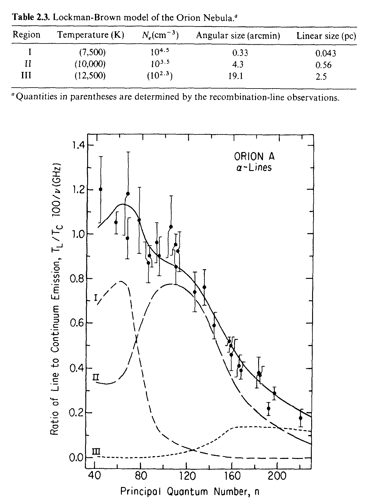
By mapping the recombination line-to-continuum ratios $T_{\mathrm{L}}/T_{\mathrm{C}}$ in a number of H $n\alpha$ transitions, Lockman and Brown determined the temperature distribution in the Orion Nebula (Figure 7.8), a nearby Hii region.

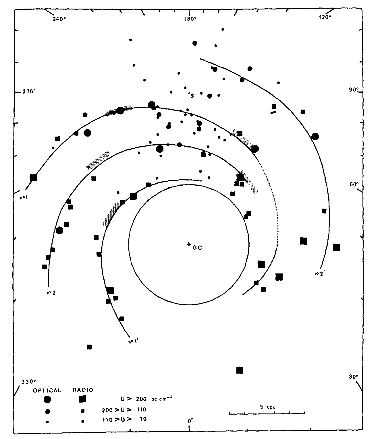
Differences between the rest and observed frequencies of radio recombination lines are attributed to Doppler shifts from nonzero radial velocities. With a simple rotational model for the disk of our Galaxy, astronomers can convert radial velocities to distances, albeit with some ambiguities, and map the approximate spatial distribution of Hii regions in our Galaxy (Figure 7.9). They roughly outline the major spiral arms.

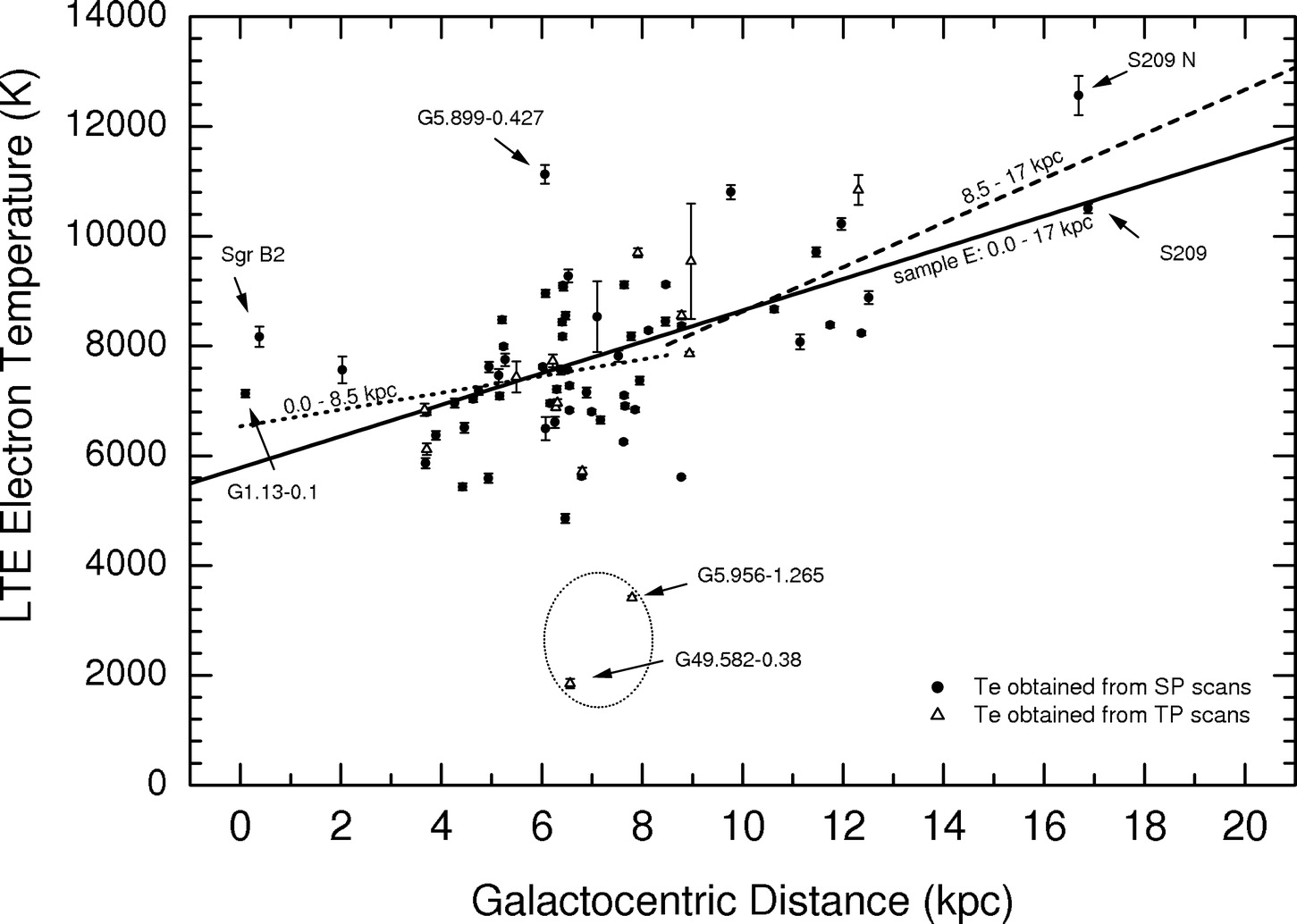
A plot showing the observed electron temperatures of Galactic Hii regions (Figure 7.10) reveals that temperature increases with distance from the Galactic center.

The explanation for this trend is the observed decrease in metallicity (relative abundance of elements heavier than helium) with galactocentric distance. Power radiated by emission lines of “metals” is the principal cause of Hii region cooling.

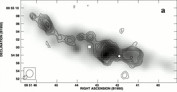
Radio recombination line strengths are much less affected by dust extinction than optical lines (e.g., the H $\alpha$ and H $\beta$ lines) are, so radio recombination lines are useful quantitative indicators of the ionization rates and hence star-formation rates in dusty starburst galaxies such as M82 (Figure 7.11).

Figure 7.11: M82 imaged in H92 $\alpha$ (contours) and 8.3 GHz continuum (gray scale) [94].

7.7 Molecular Line Spectra

7.7.1 Molecular Line Frequencies

A molecule is called polar if its permanent electric dipole moment (Equation 7.120) is not zero. Symmetric molecules (e.g., the diatomic hydrogen molecule H ${}_{2}$ ) have no permanent electric dipole moment, but most asymmetric molecules (e.g., the carbon monoxide molecule CO) do have asymmetric charge distributions and are polar. The electric dipole moments of polar molecules rotating with constant angular velocity $\omega$ appear to vary sinusoidally with that angular frequency, so polar molecules radiate at their rotation frequencies. The intensity of this radiation can be derived from the Larmor formula expressed in terms of dipole moments instead of charges and charge separations.

The permitted rotation rates and resulting line frequencies are determined by the quantization of angular momentum. The quantization rule for the permitted electron orbital radii

a_{n}=\frac{n\hbar}{m_{\mathrm{e}}v}

in the Bohr atom quantizes the orbital angular momentum $L=m_{\mathrm{e}}a_{n}v$ in multiples of $\hbar\equiv h/(2\pi)$ :

\boxed{L=n\hbar.}

(7.100)

The rule that angular momentum is an integer multiple of $\hbar$ is universal and applies to the angular momentum of a rotating molecule as well.

Consider a rigid diatomic molecule (Figure 7.12) whose two atoms have masses $m_{\mathrm{A}}$ and $m_{\mathrm{B}}$ and whose centers are separated by the equilibrium distance $r_{\mathrm{e}}$ . The individual atomic distances $r_{\mathrm{A}}$ and $r_{\mathrm{B}}$ from the center of mass must obey

r_{\mathrm{e}}=r_{\mathrm{A}}+r_{\mathrm{B}}\qquad\mathrm{and}\qquad r_{% \mathrm{A}}m_{\mathrm{A}}=r_{\mathrm{B}}m_{\mathrm{B}}.

(7.101)

Figure 7.12: A diatomic molecule rotating about its center of mass.

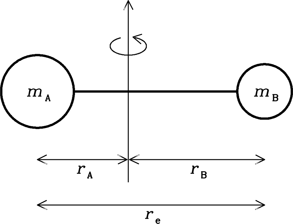
In the inertial center-of-mass frame,

L=I\omega,

(7.102)

where $I$ is the moment of inertia and $\omega$ is the angular velocity of the rotation. Nearly all of the mass is in the two compact (much smaller than $r_{\mathrm{e}}$ ) nuclei, so $I=(m_{\mathrm{A}}r_{\mathrm{A}}^{2}+m_{\mathrm{B}}r_{\mathrm{B}}^{2})$ and $L=(m_{\mathrm{A}}r_{\mathrm{A}}^{2}+m_{\mathrm{B}}r_{\mathrm{B}}^{2})\omega$ . It is convenient to rewrite this as

L=\biggl{(}\frac{m_{\mathrm{A}}m_{\mathrm{B}}}{m_{\mathrm{A}}+m_{\mathrm{B}}}% \biggr{)}r_{\mathrm{e}}^{2}\omega

(7.103)

\boxed{L=mr_{\mathrm{e}}^{2}\omega,}

(7.104)

where

\boxed{m\equiv\biggl{(}\frac{m_{\mathrm{A}}m_{\mathrm{B}}}{m_{\mathrm{A}}+m_{% \mathrm{B}}}\biggr{)}}

(7.105)

is the reduced mass of the molecule.

The rotational kinetic energy associated with this angular momentum is

E_{\mathrm{rot}}=\frac{I\omega^{2}}{2}=\frac{L^{2}}{2I}.

(7.106)

The quantization of angular momentum to integer multiples of $\hbar$ implies that rotational energy is also quantized. The corresponding energy eigenvalues of the Schrödinger equation are

\boxed{E_{\mathrm{rot}}=\biggl{(}\frac{\hbar^{2}}{2I}\biggr{)}J(J+1),\qquad J=% 0,1,2,\ldots.}

(7.107)

Note the inverse relation between permitted rotational energies and the moment of inertia $I$ . If the upper-level rotational energy is much higher than $k T$ , few molecules will be collisionally excited to that level and the line emission from molecules in that level will be very weak. For example, the minimum rotational energy of the small and light H ${}_{2}$ molecule is equivalent to a temperature $T=E_{\mathrm{min}}/k\approx 500$ K, which is much higher than the actual temperature of most interstellar H ${}_{2}$ . Only relatively massive molecules are likely to be detectable radio emitters in very cold (tens of K) molecular clouds.

Quantization of rotational energy implies that changes in rotational energy are quantized. The energy change of permitted transitions is further restricted by the quantum-mechanical selection rule

\boxed{\Delta J=\pm 1.}

(7.108)

Going from $J$ to $J-1$ releases energy

\Delta E_{\mathrm{rot}}=[J(J+1)-(J-1)J]\frac{{\hbar}^{2}}{2I}=\frac{\hbar^{2}J% }{I}.

(7.109)

The frequency of the photon emitted during this rotational transition is

\nu=\frac{\Delta E_{\mathrm{rot}}}{h}=\frac{\hbar J}{2\pi I},\qquad J=\mathrm{% 1,~{}2,}\ldots,

(7.110)

where $J$ is the angular-momentum quantum number corresponding to the upper energy level. In terms of the molecular reduced mass $m$ and equilibrium nuclear separation $r_{\mathrm{e}}$ ,

\boxed{\nu=\frac{hJ}{4\pi^{2}mr_{\mathrm{e}}^{2}},\qquad J=1,2,\ldots.}

(7.111)

Thus a plot of the radio spectrum of a particular molecular species in an interstellar cloud will look like a ladder (Figure 7.13) whose steps are all harmonics of the fundamental frequency that is determined solely by the moment of inertia $I=mr_{\mathrm{e}}^{2}$ of that species. The relative intensities of lines in the ladder depend on the temperature of the cloud. Since $\nu\propto m^{-1}r_{\mathrm{e}}^{-2}$ , the lowest frequency of line emission depends on the mass and size of the molecule. Large, heavy molecules in cold clouds may be seen at centimeter wavelengths, but smaller and lighter molecules emit only at millimeter wavelengths.

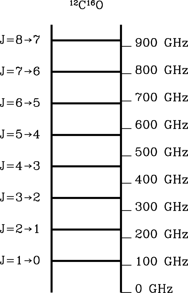
Figure 7.13: The rotational spectrum of ${}^{12}$ C ${}^{16}$ O looks like a ladder whose rungs indicate the $J$ levels and line frequencies. The ${}^{12}$ C ${}^{16}$ O molecule has a relatively small moment of inertia, so the lowest rung of this ladder is at $\nu\approx 115$ GHz ( $\lambda\approx 2.6$ mm); it has no cm-wavelength lines.

For example, the laboratory spectrum of the ${}^{12}$ C ${}^{16}$ O carbon-monoxide molecule shows that the fundamental $J=1\rightarrow 0$ transition emits a photon at $\nu=115.27120$ GHz. (See the online spectral-line catalog called Splatalogue¹¹ 1 http://www.splatalogue.net/. for accurate frequencies of radio spectral lines.) The distance $r_{\mathrm{e}}$ between the C and O nuclei can be estimated from

r_{\mathrm{e}}=\frac{1}{2\pi}\biggl{(}\frac{hJ}{m\nu}\biggr{)}^{1/2},

(7.112)

where the reduced mass is

m=\frac{m_{\mathrm{C}}m_{\mathrm{O}}}{m_{\mathrm{C}}+m_{\mathrm{O}}}\approx m_% {\mathrm{H}}\biggl{(}\frac{12\cdot 16}{12+16}\biggr{)}\approx 1.67\times 10^{-% 24}\mathrm{~{}g~{}}\cdot 6.86\approx 1.15\times 10^{-23}\mathrm{~{}g}.

Thus the equilibrium distance between the C and O nuclei is

r_{\mathrm{e}}=\frac{1}{2\pi}\biggl{(}\frac{6.63\times 10^{-27}\mathrm{~{}erg~% {}s}\cdot 1}{115.27120\times 10^{9}\mathrm{~{}Hz~{}}\cdot 1.15\times 10^{-23}% \mathrm{~{}g}}\biggr{)}^{1/2}\approx 1.13\times 10^{-8}\mathrm{~{}cm}.

The centrifugal forces acting on the nuclei increase as the molecule spins more rapidly, so a nonrigid bond will stretch and $r_{\mathrm{e}}$ will increase slightly with $J$ . Spectral lines emitted by more rapidly rotating ${}^{12}$ C ${}^{16}$ O molecules will have frequencies slightly lower than the harmonics $2\nu_{1\text{--}0},3\nu_{1\text{--}0},\ldots$ of the $J=1\rightarrow 0$ line: $2\nu_{1\text{--}0}=230.542416$ GHz and the actual $J=2\rightarrow 1$ frequency is $\nu_{2\text{--}1}=230.538000$ GHz. Chemists use these line frequencies to determine $r_{\mathrm{e}}$ , and the difference between $2\nu_{1\text{--}0}$ and $\nu_{2\text{--}1}$ is a measure of the stiffness of the carbon–oxygen chemical bond. Since the actual frequency is only slightly less than the harmonic frequency, the stiffness of the “spring” connecting the atoms is quite high. Consequently the fundamental vibrational frequency of the CO molecule is much higher than the fundamental rotational frequency, and CO emits vibrational lines at mid-infrared wavelengths $\lambda\sim 5\,\mu$ m.

Equation 7.111 can be used to calculate frequencies for molecules containing rare isotopes (e.g., ${}^{13}$ C ${}^{16}$ O) that might be more difficult to measure in the lab:

\frac{m(^{13}\mathrm{C}^{16}\mathrm{O})}{m(^{12}\mathrm{C}^{16}\mathrm{O})}=% \frac{13\cdot 16/(13+16)}{12\cdot 16/(12+16)}\approx 1.0460,

(7.113)

so we expect

	$\displaystyle\frac{\nu_{1\text{--}0}(^{13}\mathrm{C}^{16}\mathrm{O})}{\nu_{1% \text{--}0}(^{12}\mathrm{C}^{16}\mathrm{O})}\approx\biggl{[}\frac{m(^{13}% \mathrm{C}^{16}\mathrm{O})}{m(^{12}\mathrm{C}^{16}\mathrm{O})}\biggr{]}^{-1},$		(7.114)
	$\displaystyle\nu_{1\text{--}0}(^{13}\mathrm{C}^{16}\mathrm{O})\approx 115.2712% 0/1.0460\approx 110.20\mathrm{~{}GHz}.$		(7.115)

The actual ${}^{13}$ C ${}^{16}$ O $J=1\rightarrow 0$ frequency is 110.201354 GHz.

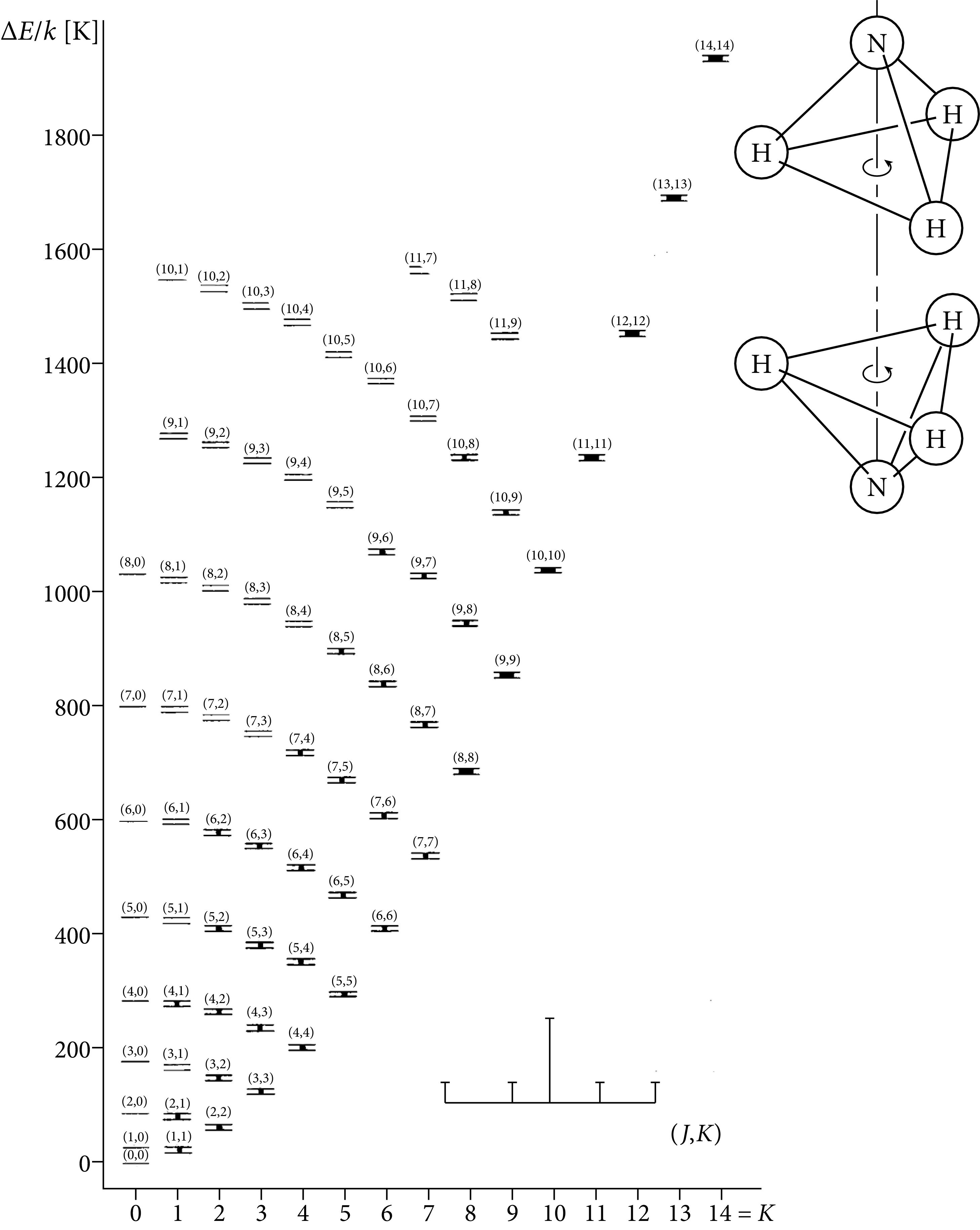
Polar diatomic molecules emit a harmonic series of radio spectral lines at millimeter wavelengths. Bigger and heavier linear polyatomic molecules have ladders of lines starting at somewhat lower frequencies. Nonlinear molecules such as the symmetric-top ammonia (NH ${}_{3}$ ) with two distinct rotational axes have more complex spectra consisting of many parallel ladders (Figure 7.14).

Figure 7.14: Energy levels of ammonia (NH ${}_{3}$ ) in the lowest vibrational state [115]. On the abscissa, $K$ is the quantum number corresponding to the $z$ -component of the angular momentum. Transitions between the two spin states of the nitrogen atom cause the line splitting shown and yield emission at frequencies near 24 GHz. NH ${}_{3}$ is a very useful thermometer for molecular clouds [52].

7.7.2 Molecular Excitation

Molecules are excited into $E_{\mathrm{rot}}>0$ states by ambient radiation and by collisions in a dense gas. The minimum gas temperature $T_{\mathrm{min}}$ needed for significant collisional excitation is

T_{\mathrm{min}}\sim\frac{E_{\mathrm{rot}}}{k}.

(7.116)

From Equations 7.107 and 7.111,

E_{\mathrm{rot}}=\frac{J(J+1)\hbar^{2}}{2I}\qquad\mathrm{and}\qquad\nu=\frac{% hJ}{4\pi^{2}I},

(7.117)

T_{\mathrm{min}}\sim\frac{J(J+1)h^{2}}{2\cdot 4\pi^{2}Ik}=\frac{hJ}{4\pi^{2}I}% \frac{h(J+1)}{2k}=\frac{E_{\mathrm{U}}}{k},

(7.118)

where $E_{\mathrm{U}}$ is the rotational energy of the upper energy level for the transition. Thus a minimum gas kinetic temperature

\boxed{T_{\mathrm{min}}\approx\frac{\nu h(J+1)}{2k}}

(7.119)

is required to excite the $J\rightarrow J-1$ transition at frequency $\nu$ . For example, the minimum gas temperature needed for significant excitation of the ${}^{12}$ C ${}^{16}$ O $J=2\text{--}1$ line at $\nu\approx 230.5$ GHz (Figure 7.15) is

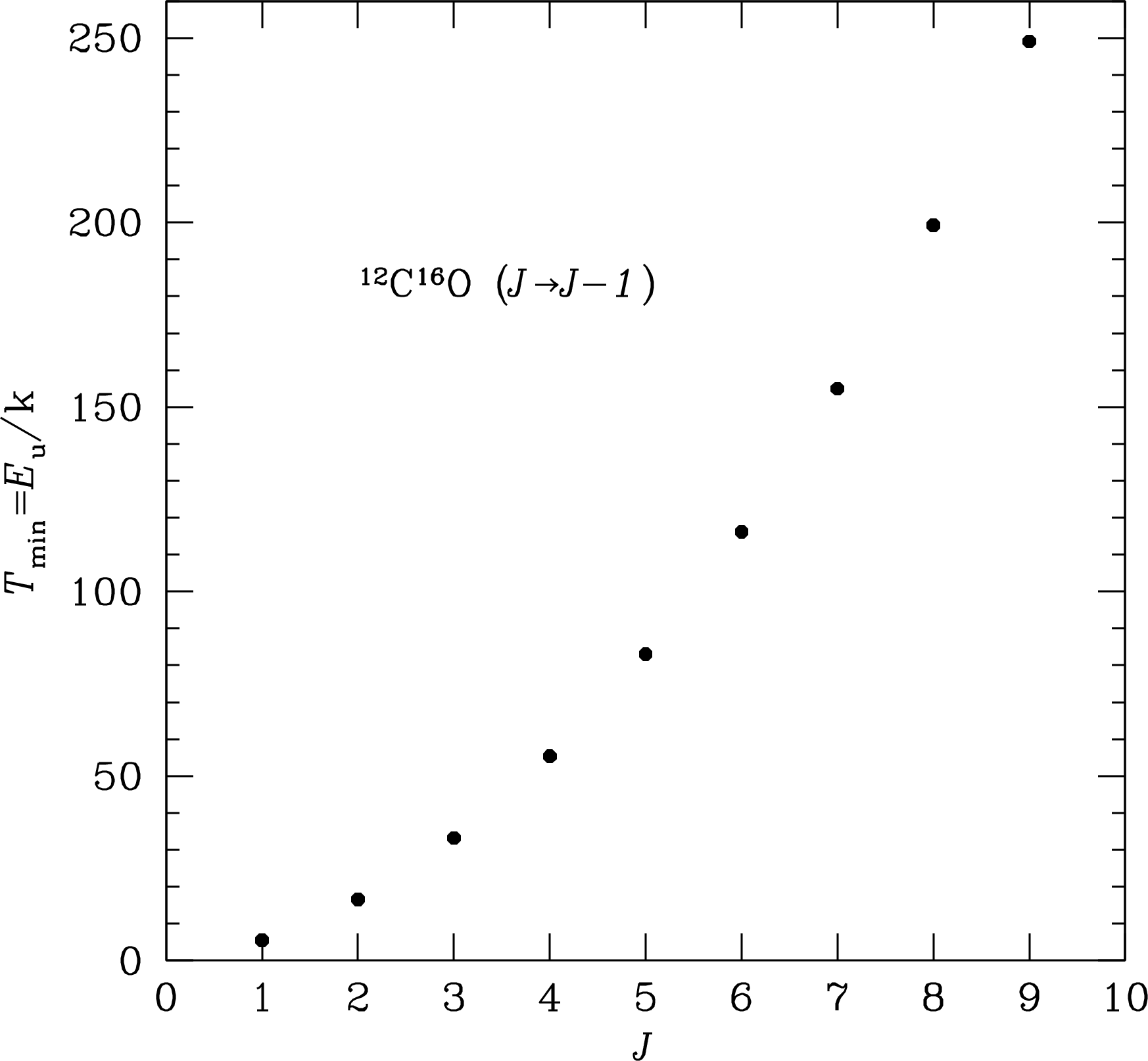
T_{\mathrm{min}}\approx\frac{\nu h(J+1)}{2k}\approx\frac{230.5\times 10^{9}% \mathrm{~{}Hz~{}}\cdot 6.63\times 10^{-27}\mathrm{~{}erg~{}s~{}}(2+1)}{2\cdot 1% .38\times 10^{-16}\mathrm{~{}erg~{}K}^{-1}}\approx 16.6\mathrm{~{}K}.

Figure 7.15: The upper-level energies $E_{\mathrm{U}}$ for ${}^{12}$ C ${}^{16}$ O $J\rightarrow J-1$ transitions are proportional to $J(J+1)$ . The corresponding minimum temperatures $T_{\mathrm{min}}=E_{\mathrm{U}}/k$ required for collisions to excite the molecules are also proportional to $J(J+1)$ , so high-J lines will be weak in cold molecular clouds.

The $T_{\mathrm{min}}=E_{\mathrm{U}}/k$ values for many molecular lines may be found in the online spectral-line catalog Splatalogue. If $T_{\mathrm{min}}\gg 2.7$ K, then radiative excitation by the cosmic microwave background is ineffective.

7.7.3 Molecular Line Strengths

Larmor’s formula for a time-varying dipole can be applied to estimate the average power radiated by a rotating polar molecule. The electric dipole moment $\vec{p}$ of any charge distribution $\rho(\vec{x})$ is defined as the integral

\vec{p}\equiv\int\vec{x}\rho(v)dv,

(7.120)

over the volume $v$ containing the charges. In the case of two point charges $+q$ and $-q$ with separation $r_{\mathrm{e}}$ ,

|\vec{p}|=qr_{\mathrm{e}}.

(7.121)

When a molecule rotates with angular velocity $\omega$ , the projection of the dipole moment perpendicular to the line of sight varies with time as $qr_{\mathrm{e}}\exp(-i\omega t)$ . Equation 7.101 states that

r_{\mathrm{A}}m_{\mathrm{A}}=r_{\mathrm{B}}m_{\mathrm{B}},

(7.122)

\dot{v}_{\mathrm{A}}=\ddot{r}_{\mathrm{A}}=\omega^{2}r_{\mathrm{A}}\qquad% \mathrm{and}\qquad\dot{v}_{\mathrm{B}}=\ddot{r}_{\mathrm{B}}=\omega^{2}r_{% \mathrm{B}}.

(7.123)

Equation 2.133 from the derivation of Larmor’s formula states that each charge contributes

E_{\bot}=\frac{q\dot{v}\sin\theta}{rc^{2}}~{}

(7.124)

to the radiated electric field at distance $r$ from the source. The fields from both charges add in phase because $r_{\mathrm{e}}\ll\lambda$ , so the total radiated field $E_{\bot}$ is

E_{\bot}=\frac{q(\omega^{2}r_{\mathrm{A}}+\omega^{2}r_{\mathrm{B}})\sin\theta}% {rc^{2}}\exp(-i\omega t).

(7.125)

Thus the instantaneous power emitted is

P=\frac{2q^{2}}{3c^{3}}\omega^{4}|r_{\mathrm{e}}\exp(-i\omega t)|^{2}

(7.126)

and the time-averaged power is

\langle P\rangle=\frac{2q^{2}}{3c^{3}}(2\pi\nu)^{4}\frac{r_{\mathrm{e}}^{2}}{2% }\,=\frac{64\pi^{4}}{3c^{3}}\nu^{4}\biggl{(}\frac{qr_{\mathrm{e}}}{2}\biggr{)}% ^{2}.

(7.127)

This can be expressed as

\langle P\rangle=\frac{64\pi^{4}}{3c^{3}}|\mu|^{2}\nu^{4},

(7.128)

where

|\mu|^{2}\equiv\biggl{(}\frac{qr_{\mathrm{e}}}{2}\biggr{)}^{2}

(7.129)

defines the mean electric dipole moment. For the radiative transition between upper and lower energy levels U and L, the spontaneous emission coefficient is

A_{\mathrm{UL}}=\frac{\langle P\rangle}{h\nu},

(7.130)

\boxed{A_{\mathrm{UL}}=\frac{64\pi^{4}}{3hc^{3}}|\mu_{\mathrm{UL}}|^{2}\nu^{3}.}

(7.131)

The value of $\mu_{\mathrm{UL}}$ for the $J\rightarrow J-1$ transition of a linear rotating molecule with dipole moment $\mu$ is

\boxed{|\mu_{\mathrm{J}\rightarrow\mathrm{J-1}}|^{2}=\frac{\mu^{2}J}{2J+1}.}

(7.132)

(This equation reflects the complex angular wave functions involved, and we won’t derive it here.)

Dipole moments are often expressed in debye units defined by $1\mathrm{~{}debye}=1\mathrm{~{}D}\equiv 10^{-18}\mathrm{~{}statcoul~{}cm}=10^{% -10}\mathrm{~{}statcoul}\times 10^{-8}\mathrm{~{}cm}$ , where $10^{-10}\mathrm{~{}statcoul}\approx 0.2\,e$ is a typical charge imbalance for a polar molecule and $10^{-8}\mathrm{~{}cm}$ is a typical value for the interatomic separation $r_{\mathrm{e}}$ . For example, the CO molecule has dipole moment $\mu\sim 0.11\times 10^{-18}\mathrm{~{}statcoul~{}cm}=0.11\mathrm{~{}D}$ .

Combining Equations 7.131 and 7.132 yields, in convenient units,

\biggl{(}\frac{A_{J\rightarrow J-1}}{\mathrm{s}^{-1}}\biggr{)}\approx 1.165% \times 10^{-11}\bigg{|}\frac{\mu}{\mathrm{D}}\bigg{|}^{2}\biggl{(}\frac{J}{2J+% 1}\biggr{)}\biggl{(}\frac{\nu}{\mathrm{GHz}}\biggr{)}^{3}.

(7.133)

For example, the spontaneous emission coefficient $A_{10}$ for the CO $J=1\rightarrow 0$ line at $\nu\approx 115$ GHz is

A_{10}\approx 1.165\times 10^{-11}\cdot 0.11^{2}\cdot\biggl{(}\frac{1}{3}% \biggl{)}\cdot 115^{3}\approx 7.1\times 10^{-8}\mathrm{~{}s}^{-1}.

(7.134)

This is close to the more accurate Splatalogue value, $A_{10}\approx 7.202\times 10^{-8}$ s ${}^{-1}$ .

The typical time $A_{10}^{-1}\approx 10^{7}$ s for a CO molecule to emit a photon spontaneously may be longer than the average time between molecular collisions in an interstellar molecular cloud, so CO can approach LTE with the excitation temperature of the $J=1\rightarrow 0$ line being nearly equal to the kinetic temperature $T$ of the molecular cloud. For any molecular transition, there is a critical density defined by

\boxed{n^{*}\approx\frac{A_{\mathrm{UL}}}{\sigma v}}

(7.135)

at which the radiating molecule suffers collisions at the rate $n^{*}\sigma v\approx n(\mathrm{H}_{2})\,\sigma v$ equal to the spontaneous emission rate $A_{\mathrm{UL}}$ . Typical collision cross sections are $\sigma\sim 10^{-15}$ cm ${}^{2}$ , and the average velocity of the abundant H ${}_{2}$ molecules is $v\approx(3kT/m)^{1/2}\sim 5\times 10^{4}$ cm s ${}^{-1}$ if $T\sim 20$ K. Thus the critical density of the CO $J=1\rightarrow 0$ transition is

n^{*}\approx\frac{A_{\mathrm{UL}}}{\sigma v}\approx\frac{7\times 10^{-8}% \mathrm{~{}s}^{-1}}{10^{-15}\mathrm{~{}cm}^{2}\cdot 5\times 10^{4}\mathrm{~{}% cm~{}s}^{-1}}\approx 1.4\times 10^{3}\mathrm{~{}cm}^{-3}.

Many Galactic molecular clouds have higher densities than this, so Galactic CO $J=1\rightarrow 0$ emission is strong and widespread. Also, photons from a particular transition may be repeatedly absorbed and reemitted within the molecular cloud. Such line trapping lowers the effective emission rate $A_{\mathrm{UL}}$ and reduces the effective value of $n^{*}$ needed for LTE.

Whether or not a molecular cloud is in LTE, Equation 7.67 with the temperature $T$ replaced by excitation temperature $T_{\mathrm{x}}$ can be used to calculate the line opacity coefficient:

\kappa(\nu)=\frac{c^{2}}{8\pi\nu_{0}^{2}}\frac{g_{\mathrm{U}}}{g_{\mathrm{L}}}% n_{\mathrm{L}}A_{\mathrm{UL}}\biggl{[}1-\exp\biggl{(}-\frac{h\nu_{0}}{kT_{% \mathrm{x}}}\biggr{)}\biggr{]}\phi(\nu).

(7.136)

At the line center frequency $\nu_{0}$ , Equation 7.37 gives

\phi(\nu_{0})=\biggl{(}\frac{\ln\,2}{\pi}\biggr{)}^{1/2}\frac{2}{\Delta\nu}=% \biggl{(}\frac{\ln\,2}{\pi}\biggr{)}^{1/2}\frac{2c}{\nu_{0}\Delta v},

where $\Delta\nu$ is the FWHM line width expressed as a frequency and $\Delta v$ is the line width in velocity units (e.g., km s ${}^{-1}$ ). The line-center optical depth is $\tau_{0}=\int\kappa_{0}\,ds$ along the line of sight, and the column density is $N_{\mathrm{L}}=\int n_{\mathrm{L}}\,ds$ along the line of sight, so

\tau_{0}=\frac{(\ln\,2)^{1/2}}{4\pi^{3/2}}\frac{c^{3}}{\nu_{0}^{3}}\frac{g_{% \mathrm{U}}}{g_{\mathrm{L}}}\frac{A_{\mathrm{UL}}}{\Delta v}N_{\mathrm{L}}% \biggl{[}1-\exp\biggl{(}-\frac{h\nu}{kT_{\mathrm{x}}}\biggr{)}\biggr{]}.

(7.137)

In the Rayleigh–Jeans approximation $h\nu\ll kT_{\mathrm{x}}$ , the brightness-temperature difference between the line center and the nearby off-line continuum is

\Delta T_{\mathrm{b}}=(T_{\mathrm{x}}-T_{\mathrm{c}})[1-\exp{(-\tau_{0})}],

(7.138)

where $T_{\mathrm{c}}$ is the brightness temperature of any background continuum emission (e.g., $T_{\mathrm{c}}\approx 2.73\mathrm{~{}K}$ from the CMB). In the limit of low line optical depth, the line brightness

\Delta T_{\mathrm{b}}\approx(T_{\mathrm{x}}-T_{\mathrm{c}})\tau_{0}=\biggl{(}% \frac{T_{\mathrm{x}}-T_{\mathrm{c}}}{T_{\mathrm{x}}}\biggr{)}N_{\mathrm{L}}% \frac{(\ln\,2)^{1/2}}{4\pi^{3/2}}\frac{hc^{3}}{k\nu_{0}^{2}}\frac{g_{\mathrm{U% }}}{g_{\mathrm{L}}}\frac{A_{\mathrm{UL}}}{\Delta v}

(7.139)

is proportional to the column density $N_{\mathrm{L}}$ . The spontaneous emission coefficient $A_{\mathrm{UL}}$ is proportional to $\nu^{3}$ (Equation 7.131), so spectral lines tend to have higher brightness temperatures and become more prominent at higher radio frequencies (Figure 7.16).

The hydrogen molecule H ${}_{2}$ is by far the most abundant molecule in interstellar space. Unfortunately, it is symmetric so its dipole moment is zero. Observable but comparatively rare polar molecules such as CO are only tracers, and total column densities of molecular gas must be estimated indirectly by the use of a fairly uncertain CO to H ${}_{2}$ conversion factor $X_{\mathrm{CO}}$ relating $H_{2}$ column density in cm ${}^{-2}$ to CO velocity-integrated line brightness in $\mathrm{K~{}km~{}s}^{-1}$ . The best current value for our Galaxy is

\boxed{X_{\mathrm{CO}}=(2\pm 0.6)\times 10^{20}\mathrm{~{}cm}^{-2}\mathrm{~{}(% K~{}km~{}s}^{-1})^{-1}.}

(7.140)

$X_{\mathrm{CO}}$ is probably higher in galaxies with low metallicity and lower in starburst galaxies [14]. Figure 8.12 shows the distribution of CO emission tracing molecular gas and obscured star formation in the interacting starburst galaxies NGC 4038/9.

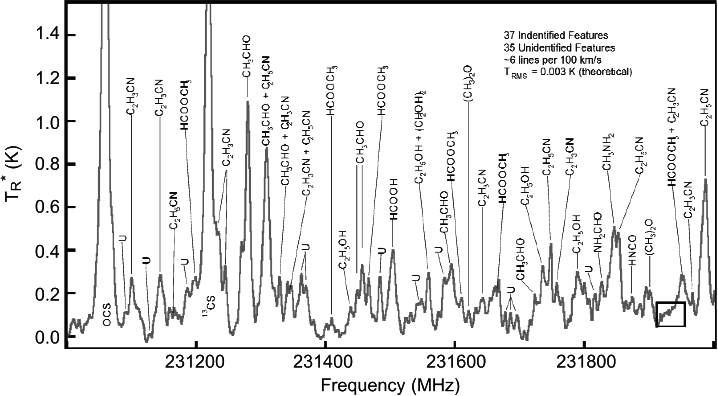
Isotopologues are molecules that differ only in isotopic composition; that is, only in the numbers of neutrons in their component atoms. Lines of the most abundant isotopologue of carbon monoxide, ${}^{12}\mathrm{C}^{16}\mathrm{O}$ , are often optically thick, so the ${}^{12}\mathrm{C}^{16}\mathrm{O}$ line brightness temperature approaches the molecular gas kinetic temperature and is nearly independent of column density. Lines of rarer isotopologues such as ${}^{13}\mathrm{C}^{16}\mathrm{O}$ or ${}^{12}\mathrm{C}^{18}\mathrm{O}$ are usually optically thin and can be used to measure the column densities needed to estimate the total mass of molecular gas in a source. Intensity ratios of optically thin lines from different $J$ levels can be used to measure excitation temperature, which is close to the kinetic temperature in LTE.

Transitions with high emission coefficients (e.g., the HCN (hydrogen cyanide) $J=1\rightarrow 0$ line at $\nu\approx 88.63$ GHz has $A_{\mathrm{UL}}\approx 2.0\times 10^{-5}$ s ${}^{-1}$ ) are collisionally excited only at very high densities ( $n^{*}\approx 10^{5}$ cm ${}^{-3}$ for HCN $J=1\rightarrow 0$ ). They are valuable for highlighting only the very dense gas directly associated with the formation of individual stars.

The discovery of ammonia (NH ${}_{3}$ ) in the direction of the Galactic center by Cheung et al. [22] immediately led to the realization that the interstellar medium must contain regions much denser than previously expected because the critical density needed to excite the NH ${}_{3}$ line is $n^{*}\approx 10^{3}$ cm ${}^{-3}$ .

Figure 7.16: This $\lambda\approx 1.3$ mm spectrum of the molecular cloud SgrB2(N) near the Galactic center is completely dominated by molecular lines from known and unknown (U) species [119]. More than 140 different molecules containing up to 13 atoms (HC ${}_{11}$ N) have been identified in space.

7.8 The Hi 21-cm Line

Hydrogen is the most abundant element in the interstellar medium (ISM), but the symmetric H ${}_{2}$ molecule has no permanent dipole moment and does not emit detectable spectral lines at radio frequencies. Neutral hydrogen (Hi) atoms are abundant and ubiquitous in low-density regions of the ISM. They are detectable in the $\lambda\approx 21$ cm ( $\nu_{10}=1420.405751\ldots$ MHz) hyperfine line. Two energy levels result from the magnetic interaction between the quantized electron and proton spins. When the relative spins change from parallel to antiparallel, a photon is emitted.

The Hi line center frequency is

\boxed{\nu_{10}=\frac{8}{3}g_{\mathrm{I}}\biggl{(}\frac{m_{\mathrm{e}}}{m_{% \mathrm{p}}}\biggr{)}\alpha^{2}(R_{M}c)\approx 1420.405751\mathrm{~{}MHz},}

(7.141)

where $g_{\mathrm{I}}\approx 5.58569$ is the nuclear $g$ -factor for a proton, $\alpha\equiv e^{2}/(\hbar c)\approx 1/137.036$ is the dimensionless fine-structure constant, and $R_{M}c$ is the hydrogen Rydberg frequency (Equation 7.12).

By analogy with the emission coefficient of radiation by an electric dipole

A_{\mathrm{UL}}\approx\frac{64\pi^{4}}{3hc^{3}}\nu_{\mathrm{UL}}^{3}|\mu_{% \mathrm{UL}}|^{2},

(7.142)

the emission coefficient of this magnetic dipole is

A_{\mathrm{UL}}\approx\frac{64\pi^{4}}{3hc^{3}}\nu_{\mathrm{UL}}^{3}|\mu_{% \mathrm{B}}|^{2},

(7.143)

where $\mu_{\mathrm{B}}$ is the mean magnetic dipole moment for Hi in the ground electronic state ( $n=1$ ). The magnitude $|\mu_{\mathrm{B}}|$ is called the Bohr magneton, and its value is

|\mu_{\mathrm{B}}|=\frac{e\hbar}{2m_{\mathrm{e}}c}\approx 9.27401\times 10^{-2% 1}\mathrm{~{}erg~{}gauss}^{-1}.

(7.144)

Thus the emission coefficient of the 21-cm line is only

	$\displaystyle A_{10}\approx\frac{64\pi^{4}(1.42\times 10^{9}\mathrm{~{}Hz})^{3% }(9.27\times 10^{-21}\mathrm{~{}erg~{}gauss}^{-1})^{2}}{3\cdot 6.63\times 10^{% -27}\mathrm{~{}erg~{}s~{}}(3\times 10^{10}\mathrm{~{}cm~{}s}^{-1})^{3}},$		(7.145)
	$\displaystyle\boxed{A_{10}\approx 2.85\times 10^{-15}\mathrm{~{}s}^{-1},}$		(7.146)

so the radiative half-life of this transition is very long:

\tau_{1/2}=A_{10}^{-1}\approx 3.5\times 10^{14}\mathrm{~{}s~{}}\approx 11% \mathrm{~{}million~{}years}.

(7.147)

Such a low emission coefficient implies an extremely low critical density (Equation 7.135) $n^{*}\ll 1\mathrm{~{}cm}^{-3}$ , so collisions can easily maintain this transition in LTE, even in the outermost regions of a normal spiral galaxy and in tidal tails of interacting galaxies.

Regardless of whether the Hi is in LTE or not, we can define the Hi spin temperature $T_{\mathrm{s}}$ (the Hi analog of the molecular excitation temperature $T_{\mathrm{x}}$ defined by Equation 7.70) by

\boxed{\frac{n_{1}}{n_{0}}\equiv\frac{g_{1}}{g_{0}}\exp\biggl{(}-\frac{h\nu_{1% 0}}{kT_{\mathrm{s}}}\biggr{)},}

(7.148)

where the statistical weights of the upper and lower spin states are $g_{1}=3$ and $g_{0}=1$ , respectively. Note that

\frac{h\nu_{10}}{kT_{\mathrm{s}}}\approx\frac{6.63\times 10^{-27}\mathrm{~{}% erg~{}s~{}}\cdot 1.42\times 10^{9}\mathrm{~{}Hz}}{1.38\times 10^{-16}\mathrm{~% {}erg~{}K}^{-1}\cdot 150\mathrm{~{}K}}\approx 5\times 10^{-4}\ll 1

(7.149)

is very small for gas in LTE at $T\approx T_{\mathrm{s}}\approx 150$ K, so in the ISM

\frac{n_{1}}{n_{0}}\approx\frac{g_{1}}{g_{0}}=3\qquad\mathrm{and}\qquad n_{% \mathrm{H}}=n_{0}+n_{1}\approx 4n_{0}.

(7.150)

Inserting these weights into Equation 7.67 gives the opacity coefficient of the $\lambda=21\mathrm{~{}cm}$ line:

	$\displaystyle\kappa(\nu)$	$\displaystyle=\frac{c^{2}}{8\pi\nu_{10}^{2}}\frac{g_{1}}{g_{0}}n_{0}A_{10}% \biggl{[}1-\exp\biggl{(}-\frac{h\nu_{10}}{kT_{\mathrm{s}}}\biggr{)}\biggr{]}% \phi(\nu)$		(7.151)
		$\displaystyle\approx\frac{c^{2}}{8\pi\nu_{10}^{2}}\cdot 3\cdot\frac{n_{\mathrm% {H}}}{4}\cdot A_{10}\biggl{(}\frac{h\nu_{10}}{kT_{\mathrm{s}}}\biggr{)}\phi(% \nu),$		(7.152)

\boxed{\kappa(\nu)\approx\frac{3c^{2}}{32\pi}\frac{A_{10}n_{\mathrm{H}}}{\nu_{% 10}}\frac{h}{kT_{\mathrm{s}}}\phi(\nu),}

(7.153)

where $n_{\mathrm{H}}$ is the number of neutral hydrogen atoms per cm ${}^{3}$ . The neutral hydrogen column density along any line of sight is defined as

\boxed{\eta_{\mathrm{H}}\equiv\int_{\mathrm{los}}n_{\mathrm{H}}(s)ds.}

(7.154)

The total opacity $\tau$ of isothermal Hi is proportional to the column density. If $\tau\ll 1$ , then the integrated Hi emission-line brightness $T_{\mathrm{b}}$ is proportional to the column density of Hi and is independent of the spin temperature $T_{\mathrm{s}}$ because $T_{\mathrm{b}}\approx T_{\mathrm{s}}\tau$ and $\tau\propto T_{\mathrm{s}}^{-1}$ in the radio limit $h\nu_{10}/(kT_{\mathrm{s}})\ll 1$ . Thus $\eta_{\mathrm{H}}$ can be determined directly from the integrated line brightness when $\tau\ll 1$ . In astronomically convenient units it can be written as

\boxed{\biggl{(}\frac{\eta_{\mathrm{H}}}{\mathrm{cm}^{-2}}\biggr{)}\approx 1.8% 2\times 10^{18}\int\biggl{[}\frac{T_{\mathrm{b}}(v)}{\mathrm{K}}\biggr{]}d% \biggl{(}\frac{v}{\mathrm{km~{}s}^{-1}}\biggr{)},}

(7.155)

where $T_{\mathrm{b}}$ is the observed 21-cm-line brightness temperature at radial velocity $v$ and the velocity integration extends over the entire 21-cm-line profile. Note that absorption by Hi in front of a continuum source with continuum brightness temperature $>T_{\mathrm{s}}$ , on the other hand, is weighted in favor of colder gas (Figure 7.17).

Figure 7.17: The Hi absorption and emission spectra toward the source 1714-397 [35].

The equilibrium temperature of cool interstellar Hi is determined by the balance of heating and cooling. The primary heat sources are cosmic rays and ionizing photons from hot stars. The main coolant in the cool atomic ISM is radiation from the fine-structure line of singly ionized carbon, Cii, at $\lambda=157.7\,\mu$ m. This line is strong only when the temperature is at least

kT\approx h\nu=\frac{hc}{\lambda},

(7.156)

so the cooling rate increases exponentially above

T\approx\frac{hc}{k\lambda}\approx\frac{6.63\times 10^{-27}\mathrm{~{}erg~{}s}% \cdot 3\times 10^{10}\mathrm{~{}cm~{}s}^{-1}}{1.38\times 10^{-16}\mathrm{~{}% erg~{}K}^{-1}\cdot 157.7\times 10^{-4}\mathrm{~{}cm}}\approx 91~{}K.

(7.157)

The actual kinetic temperature of Hi in our Galaxy can be estimated from the Hi line brightness temperatures in directions where the line is optically thick ( $\tau\gg 1$ ) and the brightness temperature approaches the excitation temperature, which is close to the kinetic temperature in LTE. Many lines of sight near the Galactic plane have brightness temperatures as high as 100–150 K, values consistent with the temperature-dependent cooling rate.

7.8.1 Galactic Hi

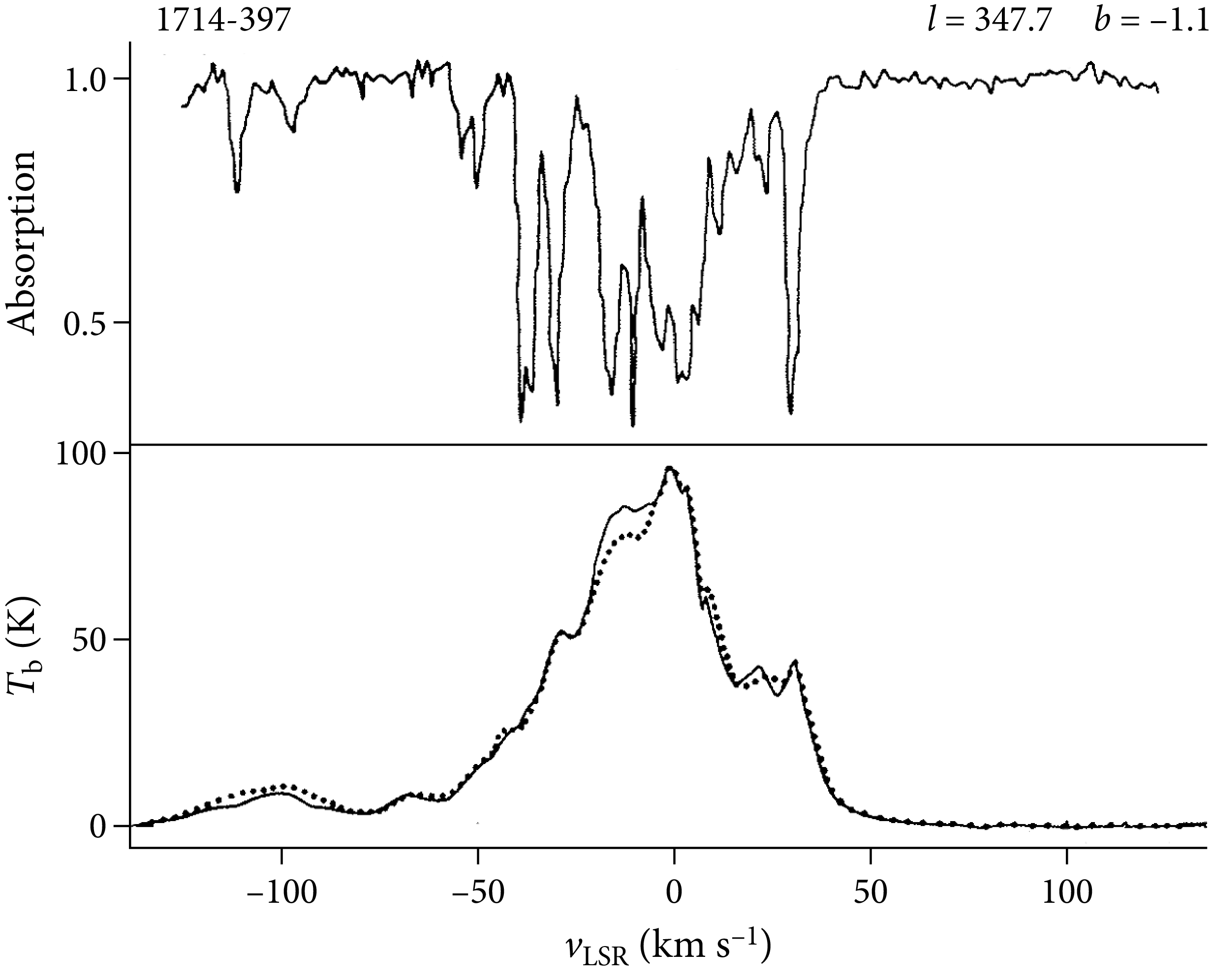
Neutral hydrogen gas in the disk of our Galaxy moves in nearly circular orbits around the Galactic center. Radial velocities $v_{r}$ measured from the Doppler shifts of Hi $\lambda=21$ cm emission lines encode information about the kinematic distances $d$ of Hi clouds, and the spectra of Hi absorption in front of continuum sources can be used to constrain their distances also. Hi is optically thin except in a few regions near the Galactic plane, so the distribution of hydrogen maps out the large-scale structure of the whole Galaxy, most of which is hidden by dust at visible wavelengths.

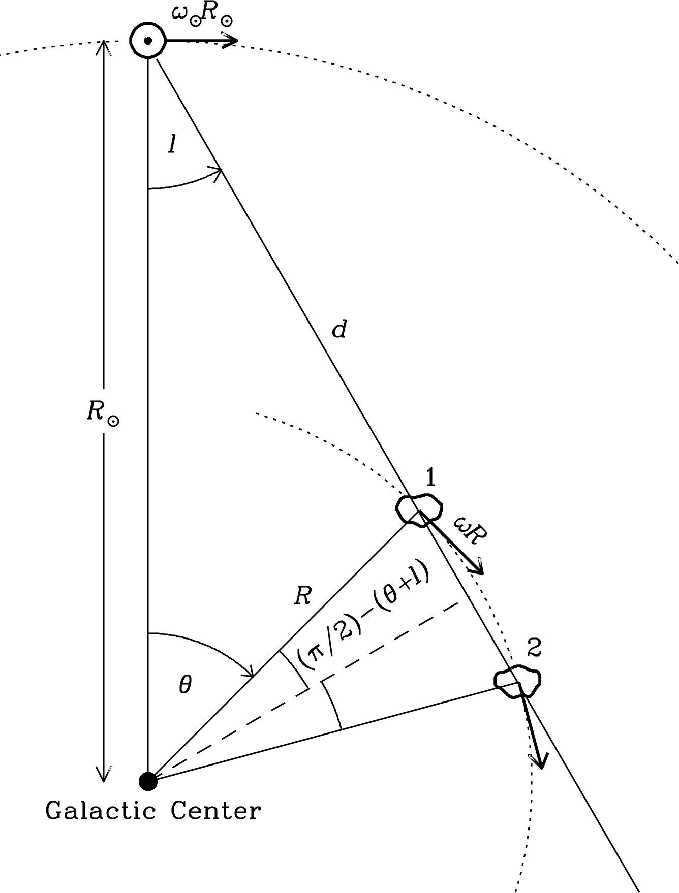
Figure 7.18: In the simplest realistic model for the Galactic disk, the Sun and all Hi clouds are in circular orbits about the Galactic center, and the angular orbital velocity $\omega$ is a monotonically decreasing function of the orbital radius $R$ . The distance of the Sun from the Galactic center is $R_{\odot}=8.0\pm 0.5$ kpc, and the Sun’s orbital speed is $\omega_{\odot}R_{\odot}\approx 220$ km s ${}^{-1}$ . The angle $l$ defines the Galactic longitude. For $|l|<\pi/2$ , two Hi clouds (1 and 2) can have the same radial velocity but be at different distances from the Sun.

Figure 7.18 shows a plan view of the Galactic disk. The Sun ( $\odot$ ) lies in the disk and moves in a circular orbit around the Galactic center. The distance to the Galactic center $R_{\odot}=8.0\pm 0.5$ kpc and the Sun’s orbital speed $\omega_{\odot}R_{\odot}\approx 220$ km s ${}^{-1}$ have been measured by a variety of means [90]. All Hi clouds at galactocentric distance $R$ are assumed to be in circular orbits with angular velocity $\omega(R)$ , where $\omega(R)$ is a monotonically decreasing function of $R$ . For cloud 1 at galactocentric azimuth $\theta$ on the line of sight at Galactic longitude $l$ , the observed radial velocity $v_{r}$ relative to the Sun is given by

v_{r}=\omega R\cos[\pi/2-(l+\theta)]-\omega_{\odot}R_{\odot}\cos(\pi/2-l).

(7.158)

Using the trigonometric identities $\cos[\pi/2-(l+\theta)]=\sin(l+\theta)$ and $\sin(l+\theta)=\sin\theta\cos l+\cos\theta\sin l$ we obtain

	$\displaystyle v_{r}$	$\displaystyle=\omega R(\sin\theta\cos l+\cos\theta\sin l)-\omega_{\odot}R_{% \odot}\sin l$		(7.159)
		$\displaystyle=R_{\odot}(\omega-\omega_{\odot})\sin l.$		(7.160)

To apply this equation, we need to determine the rotation curve $R\omega(R)$ . The maximum radial velocity on the line of sight at longitude $l$ is called the “terminal velocity” $v_{\mathrm{T}}$ . Since $\omega$ decreases with $R$ , this velocity occurs at the minimum $R=R_{\mathrm{min}}=R_{\odot}\sin l$ where the orbit is tangent to the line of sight:

v_{\mathrm{T}}=R_{\odot}[\omega(R_{\mathrm{min}})-\omega_{\odot}]\sin l.

(7.161)

We can determine the rotation curve from measurements of $v_{\mathrm{T}}$ spanning a wide range of $l$ and thus of $R_{\mathrm{min}}$ .

Example. At Galactic longitude

l=30^{\circ}

, the terminal velocity is observed to be

v_{\mathrm{T}}\approx 130

km s

{}^{-1}

. What is

R_{\mathrm{min}}

and the orbital speed

R_{\mathrm{min}}\omega(R_{\mathrm{min}})

\displaystyle R_{\mathrm{min}}

\displaystyle=R_{\odot}\sin l=8.0\mathrm{~{}kpc}\cdot 0.5=4.0\mathrm{~{}kpc},

\displaystyle v_{\mathrm{T}}

\displaystyle=R_{\odot}[\omega(R_{\mathrm{min}})-\omega_{\odot}]\sin l

\displaystyle=R_{\mathrm{min}}\omega(R_{\mathrm{min}})-R_{\odot}\omega_{\odot}% \sin l,

\displaystyle R_{\mathrm{min}}\omega(R_{\mathrm{min}})

\displaystyle=v_{\mathrm{T}}+R_{\odot}\omega_{\odot}\sin l

\displaystyle=130\mathrm{~{}km~{}s}^{-1}+220\mathrm{~{}km~{}s}^{-1}\cdot 0.5=2% 40\mathrm{~{}km~{}s}^{-1}.

Beware that, for

|l|<\pi/2

, there is a distance ambiguity: clouds 1 and 2 have the same radial velocity but different distances

d

. There is no distance ambiguity for

|l|>\pi/2

7.8.2 Hi in External Galaxies

The 1420 MHz Hi line is an extremely useful tool for studying gas in the ISM of external galaxies and tracing the large-scale distribution of galaxies in the universe because Hi is detectable in most spiral galaxies and in some elliptical galaxies.

Because $\lambda=21$ cm is such a long wavelength, many galaxies are unresolved by single-dish radio telescopes. For example, the half-power beamwidth of the 100-m GBT is about 9 arcmin at $\lambda=21$ cm. Thus a single pointing is sufficient to obtain a spectral line representing all of the Hi in any but the nearest galaxies.

The observed center frequency of the Hi line can be used to measure the radial velocity $v_{r}$ of a galaxy. The radial velocity of a galaxy is the sum of the recession velocity caused by the uniform Hubble expansion of the universe and the “peculiar” velocity of the galaxy. The radial component of the peculiar velocity reflects motions caused by gravitational interactions with nearby galaxies and is typically $\sim 200$ km s ${}^{-1}$ in magnitude. The Hubble velocity is proportional to distance from the Earth, and the Hubble constant of proportionality has been measured as $H_{0}=67.8\pm 0.9\mathrm{~{}km~{}s}^{-1}\mathrm{~{}Mpc}^{-1}$ [83]. If the radial velocity is significantly larger than the radial component of the peculiar velocity, the observed Hi frequency can be used to estimate the distance $d\approx v_{r}/H_{0}$ to a galaxy.

Beware that astronomers still use inconsistent radial velocity conventions that were established when most observed radial velocities were much less than the speed of light. The approximation

\frac{v_{r}}{c}\approx\frac{\nu_{\mathrm{e}}-\nu_{\mathrm{o}}}{\nu_{\mathrm{e}% }}\qquad(v_{r}\ll c),

(7.162)

where $\nu_{\mathrm{e}}$ is the line frequency in the source frame and $\nu_{\mathrm{o}}$ is the observed frequency, was used to define the radio velocity for any $v_{r}(\mathrm{radio})$ as

v_{r}(\mathrm{radio})\equiv c\biggl{(}\frac{\nu_{\mathrm{e}}-\nu_{\mathrm{o}}}% {\nu_{\mathrm{e}}}\biggr{)}

(7.163)

because radio astronomers measure frequencies, not wavelengths. Optical astronomers measure wavelengths, not frequencies, so the nonrelativistic approximation

\frac{v_{r}}{c}\approx\frac{\lambda_{\mathrm{o}}-\lambda_{\mathrm{e}}}{\lambda% _{\mathrm{e}}}\qquad(v_{r}\ll c)

(7.164)

is the basis for the optical velocity defined for any $v_{r}(\mathrm{optical})$ by

v_{r}(\mathrm{optical})\equiv c\biggl{(}\frac{\lambda_{\mathrm{o}}-\lambda_{% \mathrm{e}}}{\lambda_{\mathrm{e}}}\biggr{)}=cz,

(7.165)

where $z$ is the redshift defined by Equation 2.127. The optical and radio velocity conventions are not exactly the same, and neither agrees with the relativistically correct radial velocity calculated from Equation 5.142. Occasionally an observer confuses velocity conventions, fails to center the observing passband on the correct frequency, and ends up with only part of the Hi spectrum of a galaxy. Outside the local universe ( $z\ll 1$ ) the concept of distance itself becomes more complicated. To calculate distances to astronomical objects with larger redshifts, see Hogg [53, “Distance measures in cosmology”].

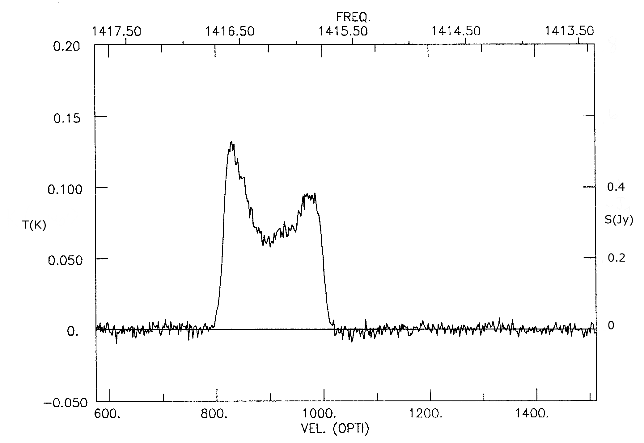
Figure 7.19: This integrated Hi spectrum of UGC 11707 was obtained by Haynes et al. [47] with the 140-foot telescope (beamwidth $\approx 20$ arcmin) and shows the typical two-horned profile of a spiral galaxy. The velocity axis is clearly labeled as showing the “optical” velocity.

For example, the Hi emission-line profile (Figure 7.19) of the galaxy UGC 11707 can be used to estimate its distance $d\approx v_{r}/H_{0}$ . The observed line center frequency is $\nu_{\mathrm{o}}\approx 1416.2$ MHz, so the “radio” and “optical” velocities are

	$\displaystyle v_{r}(\mathrm{radio})$	$\displaystyle\approx$	$\displaystyle c\biggl{(}1-\frac{\nu_{\mathrm{o}}}{\nu_{\mathrm{e}}}\biggr{)}% \approx 3\times 10^{5}\mathrm{~{}km~{}s}^{-1}\biggl{(}1-\frac{1416.2\mathrm{~{% }MHz}}{1420.4\mathrm{~{}MHz}}\biggr{)}\approx 890\mathrm{~{}km~{}s}^{-1},$
	$\displaystyle v_{r}(\mathrm{optical})$	$\displaystyle\approx$	$\displaystyle c\biggl{(}\frac{\nu_{\mathrm{e}}}{\nu_{\mathrm{o}}}-1\biggr{)}% \approx 3\times 10^{5}\mathrm{~{}km~{}s}^{-1}\biggl{(}\frac{1420.4\mathrm{~{}% MHz}}{1416.2\mathrm{~{}MHz}}-1\biggr{)}\approx 889\mathrm{~{}km~{}s}^{-1}.$

Using the “optical” velocity gives

d\approx\frac{v_{r}(\mathrm{optical})}{H_{0}}\approx\frac{889\mathrm{~{}km~{}s% }^{-1}}{67.8\mathrm{~{}km~{}s}^{-1}\mathrm{~{}Mpc}^{-1}}\approx 13\mathrm{~{% }Mpc}.

If the Hi emission from a galaxy is optically thin, then the integrated line flux is proportional to the mass of Hi in the galaxy, independent of the unknown Hi temperature. It is a straightforward exercise to derive from Equation 7.155 the relation

\boxed{\biggl{(}\frac{M_{\mathrm{H}}}{M_{\odot}}\biggr{)}\approx 2.36\times 10% ^{5}\biggl{(}\frac{d}{\mathrm{Mpc}}\biggr{)}^{2}\int\biggl{[}\frac{S(v)}{% \mathrm{Jy}}\biggr{]}\biggl{(}\frac{dv}{\mathrm{km~{}s}^{-1}}\biggr{)}}

(7.166)

for the total Hi mass $M_{\mathrm{H}}$ of a galaxy. The integral $\int S(v)dv$ over the line is called the line flux and is usually expressed in units of Jy km s ${}^{-1}$ . For example, to estimate the Hi mass of UGC 11707, assume $\tau\ll 1$ . The single-dish Hi line profile of UGC 11707 (Figure 7.19) indicates a line flux

\int S(v)dv\approx 0.35\mathrm{~{}Jy}\cdot 200\mathrm{~{}km~{}s}^{-1}\approx 7% 0\mathrm{~{}Jy~{}km~{}s}^{-1},

\biggl{(}\frac{M_{\mathrm{H}}}{M_{\odot}}\biggr{)}\approx 2.36\times 10^{5}% \cdot(13)^{2}\cdot 70\approx 2.8\times 10^{9}.

Small statistical corrections for nonzero $\tau$ can be made from knowledge about the expected opacity as a function of disk inclination, galaxy mass, morphological type, etc.

A well-resolved Hi image of a galaxy yields the total mass $M(r)$ enclosed within radius $r$ of the center if the gas orbits in circular orbits.

If the mass distribution of every galaxy were spherically symmetric, the gravitational force at radius $r$ would equal the gravitational force of the enclosed mass $M(r)$ . This is not a bad approximation, even for disk galaxies. Thus for gas in a circular orbit with orbital velocity $v_{\mathrm{rot}}$ ,

\frac{GM}{r^{2}}=\frac{v_{\mathrm{rot}}^{2}}{r},

(7.167)

where $M$ is the mass enclosed within the sphere of radius $r$ and $v$ is the orbital velocity at radius $r$ , so

v_{\mathrm{rot}}^{2}=\frac{GM}{r}.

(7.168)

Note that the velocity $v_{\mathrm{rot}}$ is the full rotational velocity, not just its radial component $v_{\mathrm{rot}}\sin i$ , where $i$ is the inclination angle between the galaxy disk and the line of sight. The inclination angle of a thin circular disk can be estimated from the axial ratio

\cos i=\frac{\theta_{\mathrm{m}}}{\theta_{\mathrm{M}}},

(7.169)

where $\theta_{\mathrm{m}}$ and $\theta_{\mathrm{M}}$ are the minor- and major-axis angular diameters, respectively. Converting from CGS to astronomically convenient units yields

$\displaystyle\biggl{[}\biggl{(}\frac{v_{\mathrm{rot}}}{\mathrm{cm~{}s}^{-1}}% \biggr{)}\biggl{(}\frac{10^{5}\mathrm{~{}cm~{}s}^{-1}}{\mathrm{km~{}s}^{-1}}% \biggr{)}\biggr{]}^{2}$	$\displaystyle=\biggl{[}6.67\times 10^{-8}\mathrm{~{}dyne~{}cm}^{2}\mathrm{~{}g% }^{-2}\cdot\biggl{(}\frac{M}{\mathrm{g}}\biggr{)}\biggl{(}\frac{2\times 10^{33% }\mathrm{~{}g}}{M_{\odot}}\biggr{)}\biggr{]}$
	$\displaystyle\quad\times\biggl{[}\biggl{(}\frac{r}{\mathrm{cm}}\biggr{)}\biggl% {(}\frac{3.09\times 10^{21}\mathrm{~{}cm}}{\mathrm{kpc}}\biggr{)}\biggr{]}^{-1},$	(7.170)
$\displaystyle 10^{10}\biggl{(}\frac{v_{\mathrm{rot}}}{\mathrm{km~{}s}^{-1}}% \biggr{)}^{2}$	$\displaystyle=\biggl{[}6.67\times 10^{-8}\cdot 2\times 10^{33}\biggl{(}\frac{M% }{M_{\odot}}\biggr{)}\biggr{]}$
	$\displaystyle\quad\times\biggl{[}3.09\times 10^{21}\biggl{(}\frac{r}{\mathrm{% kpc}}\biggr{)}\biggr{]}^{-1},$	(7.171)

and we obtain the total galaxy mass inside radius $r$ in units of the solar mass:

\boxed{\biggl{(}\frac{M}{M_{\odot}}\biggr{)}\approx 2.3\times 10^{5}\biggl{(}% \frac{v_{\mathrm{rot}}}{\mathrm{km~{}s}^{-1}}\biggr{)}^{2}\biggl{(}\frac{r}{% \mathrm{kpc}}\biggr{)}.}

(7.172)

Thus the total mass of UGC 11707 (Figure 7.20) can be estimated from

	$\displaystyle v_{\mathrm{rot}}\sin i$	$\displaystyle\approx\frac{\Delta v_{\mathrm{rot}}\sin i}{2}\approx\frac{(1000% \mathrm{~{}km~{}s}^{-1}-800\mathrm{~{}km~{}s}^{-1})}{2}\approx 100\mathrm{~{}% km~{}s}^{-1},$
	$\displaystyle\cos i$	$\displaystyle\approx\frac{\mathrm{minor~{}axis}}{\mathrm{major~{}axis}}\approx% \frac{0.73\times 10^{-3}\mathrm{~{}rad}}{2.0\times 10^{-3}\mathrm{~{}rad}}% \approx 0.365,\qquad\mathrm{so}\qquad\sin i\approx 0.93,$
	$\displaystyle r$	$\displaystyle\approx\theta_{1/2}d\approx 10^{-3}\mathrm{~{}rad~{}}\cdot 13% \mathrm{~{}Mpc}\approx 13\mathrm{~{}kpc},$
so
	$\displaystyle\biggl{(}\frac{M}{M_{\odot}}\biggr{)}$	$\displaystyle\approx 2.3\times 10^{5}\cdot(100/0.93)^{2}\cdot 13=3.5\times 1% 0^{10}.$

UGC 11707 is a relatively low-mass spiral galaxy.

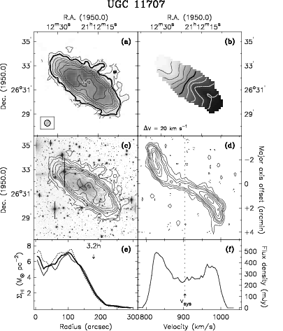
Figure 7.20: Hi images of UGC 11707 [104]. The hatched circle in the lower left corner of panel (a) shows the image resolution. The contours in panels (a) and (c) outline the integrated Hi brightness distribution. Panel (b) shows contours of constant velocity separated by 20 km s ${}^{-1}$ and the darker shading indicates approaching gas. Panel (d) is a position-velocity diagram, panel (e) is the radial Hi column-density profile, and panel (f) displays the integrated Hi spectrum.

This “total” mass is really only the mass inside the radius sampled by detectable Hi. Even though Hi extends beyond most other tracers such as molecular gas or stars, it is clear from plots of Hi rotation velocities versus radius that not all of the mass is being sampled, because we don’t see the Keplerian relation $v_{\mathrm{rot}}\propto r^{-1/2}$ which indicates that all of the mass is enclosed within radius $r$ . Most rotation curves, one-dimensional position-velocity diagrams along the major axis, are flat at large $r$ , suggesting that the enclosed mass $M\propto r$ as far as we can see Hi. The large total masses implied by Hi rotation curves provided some of the earliest evidence for the existence of cold dark matter in galaxies.

Because detectable Hi is so extensive, Hi is an exceptionally sensitive tracer of tidal interactions between galaxies. Long streamers and tails of Hi trace the interaction histories of pairs and groups of galaxies. See Figure 8.11 showing Hi in the M81 group of galaxies and Figure 8.12 revealing long tidal tails of Hi from the “Antennae” galaxy pair NGC 4038/9.

Another application of the Hi spectra of galaxies is determining departures from smooth Hubble expansion in the local universe via the Tully–Fisher relation. Most galaxies obey the empirical luminosity–velocity relation [108]:

L\propto v_{\mathrm{m}}^{4},

(7.173)

where $v_{\mathrm{m}}$ is the maximum rotation speed. Arguments based on the virial theorem can explain the Tully–Fisher relation if all galaxies have the same central mass density and density profile, differing only in scale length, and also have the same mass-to-light ratio. Thus a measurement of $v_{\mathrm{m}}$ yields an estimate of $L$ that is independent of the Hubble distance $d_{\mathrm{H}}$ . The Tully–Fisher distance $d_{\mathrm{TF}}$ can be calculated from this “standard candle” $L$ and the apparent luminosity. Apparent luminosities in the near infrared ( $\lambda\sim 2\,\mu$ m) are favored because the near-infrared mass-to-light ratio of stars is nearly constant and independent of the star-formation history, and because extinction by dust is much less than at optical wavelengths. Differences between $d_{\mathrm{TF}}$ and $d_{\mathrm{H}}$ are ascribed to the peculiar velocities of galaxies caused by intergalactic gravitational interactions. The magnitudes and scale lengths of the peculiar velocity distributions are indications of the average density and clumpiness of mass on megaparsec scales.

7.8.3 Dark Ages and the Epoch of Reionization (EOR)

Most of the baryonic matter in the early universe was fully ionized hydrogen and helium gas, plus trace amounts of heavier elements. This smoothly distributed gas cooled as the universe expanded, and the free protons and electrons recombined to form neutral hydrogen at a redshift $z\approx 1091$ when the age of the universe was about $3.8\times 10^{5}$ years. The hydrogen remained neutral during the dark ages prior to the formation of the first ionizing astronomical sources—massive ( $M>100M_{\odot}$ ) stars, galaxies, quasars, and clusters of galaxies—by gravitational collapse of overdense regions. These astronomical sources gradually started reionizing the universe when it was several hundred million years old ( $z\sim 10$ ) and completely reionized the universe by the time it was about $10^{9}$ years old ( $z\sim 6$ ). This era is called the epoch of reionization.

The highly redshifted Hi signal was nearly uniform during the dark ages, and it developed structure on angular scales up to several arcmin when the first astronomical sources created bubbles of ionized hydrogen around them. As the bubbles grew and merged, the Hi signal developed frequency structure corresponding to the redshifted Hi line frequency. The characteristic size of the larger bubbles reached about 10 Mpc at $z\sim 6$ and produced Hi signals having angular scales of several arcmin and covering frequency ranges of several MHz. These Hi signals encode unique information about the formation of the earliest astronomical sources.

The Hi signals produced by the EOR will be very difficult to detect because they are weak (tens of mK), relatively broad in frequency, redshifted to low frequencies ( $\sim 100$ MHz) plagued by radio-frequency interference and ionospheric refraction, and lie behind a much brighter (tens of K) foreground of extragalactic continuum radio sources. Nonetheless, the potential scientific payoff is so great that several groups around the world are developing instruments to detect the Hi signature of the EOR. Two such instruments are PAPER (Precision Array to Probe the Epoch of Reionization) [79] and the Murchison Widefield Array [54] shown in Figure 8.7.