Next: A Computer-Based Technique for Automatic Description and
Classification of Newly-Observed Data
Previous: Variable-Pixel Linear Combination
Up: Algorithms
Table of Contents - Index - PS reprint
Astronomical Data Analysis Software and Systems VI
ASP Conference Series, Vol. 125, 1997
Editors: Gareth Hunt and H. E. Payne
James Theiler and Jeff Bloch
Astrophysics and Radiation Measurements Group, MS-D436
Los Alamos National Laboratory, Los Alamos, NM 87545
e-mail:
jt@lanl.gov,
jbloch@lanl.gov
Abstract:
The ALEXIS
(Array of Low Energy X-ray Imaging Sensors) (Priedhorsky et al. 1989)
satellite scans nearly half the sky every fifty seconds, and downlinks
time-tagged photon data twice a day. The standard science quicklook
processing produces over a dozen sky maps at each downlink, and these maps
are automatically searched for potential transient point sources. We are
interested only in highly significant point source detections,
and, based on earlier Monte-Carlo studies (Roussel-Dupré et al. 1996),
only consider p<10-7, which is about 5.2 ``sigmas.'' Our algorithms
are therefore required to operate on the far tail of the distribution,
where many traditional approximations break down. Although an exact
solution is available for the case of unweighted counts (Lampton 1994),
the problem is more difficult in the case of weighted counts. We have
found that a heuristic modification of a formula derived by Li & Ma
(1983) provides reasonably accurate estimates of p-values for point
source detections even for very low p-value detections.
We test the null hypothesis of no point source (assuming a
spatially uniform background) at a given location by enclosing that
location with a source kernel (whose area  is generally matched
to the point-spread-function of the telescope) and then
enclosing the source kernel with a relatively large background annulus
(area
is generally matched
to the point-spread-function of the telescope) and then
enclosing the source kernel with a relatively large background annulus
(area  ). Given
  photons in the source kernel, and
 photons in the background annulus, the problem is to determine
whether the number of source photons is significantly larger
than expected under the null.
photons in the background annulus, the problem is to determine
whether the number of source photons is significantly larger
than expected under the null.
More sensitive point source detection is obtained by weighting the
photons to match the point-spread function of the
telescope more precisely. Further enhancements are obtained for ALEXIS data by
weighting also according to instantaneous scalar background rate,
pulse height, and position on the detector. In this case, we ask
whether the weighted sum of photons in the source region is
significantly larger than expected under the null.
If counts are unweighted (i.e., all weights are equal), then it
is possible to write down an exact, explicit expression for the
probability of seeing  or more photons in the source kernel,
assuming
or more photons in the source kernel,
assuming 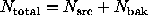 is fixed. This is a binomial
distribution, and Lampton (1994) showed that the p-value associated
with this observation can be expressed in terms of the incomplete beta
function:
is fixed. This is a binomial
distribution, and Lampton (1994) showed that the p-value associated
with this observation can be expressed in terms of the incomplete beta
function:  , where
  . See
also Alexandreas et al. (1994), for an alternative derivation of
an equivalent expression (the assumption that
. See
also Alexandreas et al. (1994), for an alternative derivation of
an equivalent expression (the assumption that  is fixed is
replaced by a Bayesian argument).
is fixed is
replaced by a Bayesian argument).
If the count rate is high (or the exposure long), so that  and
and
 are large, then an appropriate Gaussian approximation can be used.
In general, this involves finding a ``signal'' and dividing it by
the square root of its variance.
are large, then an appropriate Gaussian approximation can be used.
In general, this involves finding a ``signal'' and dividing it by
the square root of its variance.
Case 1u. The most straightforward approach uses
the signal  , where
  .
Under the null hypothesis, this signal has an expected value of zero, and
a variance-if
.
Under the null hypothesis, this signal has an expected value of zero, and
a variance-if  and
and  are treated as independent Poisson
sources-of
are treated as independent Poisson
sources-of 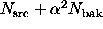 . To get a p-value, use

where 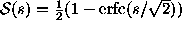 converts
``sigmas'' of significance into a one-tailed p-value.
converts
``sigmas'' of significance into a one-tailed p-value.
Case 2u. An alternative approach, suggested by Li & Ma (1983),
treats the sum  ,
as fixed, so that
,
as fixed, so that  and
and  are binomially distributed. In
particular, choose the signal
are binomially distributed. In
particular, choose the signal 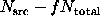 , and note that the
variance of
, and note that the
variance of  is given by
 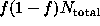 , while the variance of
 is by definition zero. In that case
Case 3u.
By looking at a ratio of Poisson likelihoods, Li & Ma (1983) also derived
a more complicated equation

where  and
and  . This is
considerably more accurate than Eqs. (14,15) when
. This is
considerably more accurate than Eqs. (14,15) when
 and
and  are not large, but is still just an approximation to
Lampton's exact formula. Abramowitz & Stegun (1972) provide several
approximations to the incomplete beta function, one of which (25.5.19) is an
asymptotic series whose first term looks very much like the Li & Ma
formula.
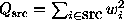
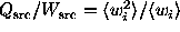
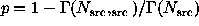
The left panel of Figure 1 compares these cases, along
with the Lampton (1994) formula, using a Monte-Carlo simulation.
are not large, but is still just an approximation to
Lampton's exact formula. Abramowitz & Stegun (1972) provide several
approximations to the incomplete beta function, one of which (25.5.19) is an
asymptotic series whose first term looks very much like the Li & Ma
formula.
The left panel of Figure 1 compares these cases, along
with the Lampton (1994) formula, using a Monte-Carlo simulation.
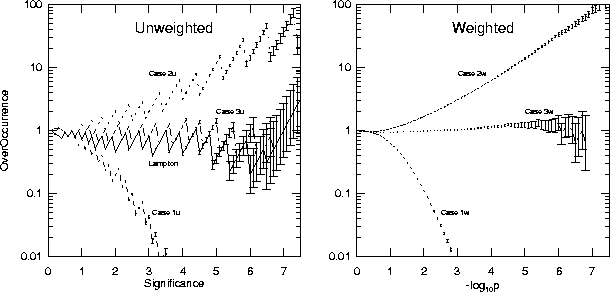
Figure: Results of Monte-Carlo experiments with N=100 photons, with
 , and with
  trials. For the weighted experiment,
N weights were uniformly chosen from zero to one,
and assigned to the N photons. The photons
were randomly assigned to the source kernel or background annulus with
probabilities f and 1-f respectively. Values of
trials. For the weighted experiment,
N weights were uniformly chosen from zero to one,
and assigned to the N photons. The photons
were randomly assigned to the source kernel or background annulus with
probabilities f and 1-f respectively. Values of  ,
,  ,
,
 , and
, and  were computed, and a p-value was computed using
the formulas for the three cases.
As the p-values were computed, a cumulative histogram
were computed, and a p-value was computed using
the formulas for the three cases.
As the p-values were computed, a cumulative histogram  was
built indicating the number of times a p-value less than p was observed.
Since we expect
was
built indicating the number of times a p-value less than p was observed.
Since we expect  , we plotted
  as the frequency of
``overoccurrence'' of that p-value. The plot is this overoccurrence
as a function of ``significance,'' defined by
as the frequency of
``overoccurrence'' of that p-value. The plot is this overoccurrence
as a function of ``significance,'' defined by  .
Original PostScript figure (87kB).
.
Original PostScript figure (87kB).
Define 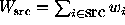 and
and
 , where
  is the weight of the
i-th photon. Notice
that when all the weights are equal to one, we have
is the weight of the
i-th photon. Notice
that when all the weights are equal to one, we have
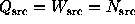 and
and 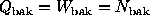 . Note
also that
. Note
also that 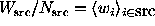 , and that
 . We do not
make any assumptons about weights averaging or summing to unity. (We
define
. We do not
make any assumptons about weights averaging or summing to unity. (We
define  and
and  similarly.)
Generalizing Case 1u, we define the signal as  and
then treating source and background as independent, we can write the
variance as
and
then treating source and background as independent, we can write the
variance as 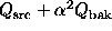 . We can similarly generalize Case 2u
and obtain:
. We can similarly generalize Case 2u
and obtain:
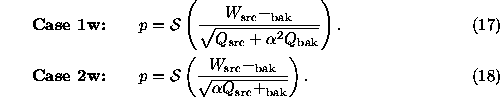
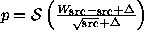
Case 3w:
It is not as straightforward to generalize Eq. (16), but we have
tried the following heuristic:

where  and
and 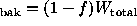 .
The Monte-Carlo results shown in Figure 1 indicate that this
heuristic provides reasonably accurate p-values even for very small
values of p.
.
The Monte-Carlo results shown in Figure 1 indicate that this
heuristic provides reasonably accurate p-values even for very small
values of p.
An interesting limit occurs as the background annulus becomes large. Here,
 , and the expected
backgrounds
, and the expected
backgrounds  ,
,  , etc. are all precisely known.
For the unweighted counts, the exact p-value can be expressed
in terms of the incomplete gamma function:
 . The
Gaussian estimate of significance is straightforward
. The
Gaussian estimate of significance is straightforward both for the unweighted case,
  , and for the weighted
case:
, and for the weighted
case: 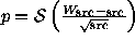 .
In this limit, Eq. (19) becomes
.
In this limit, Eq. (19) becomes

Marshall (1994) has suggested an empirical formula
 ,
where
,
where 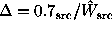 , which produced reasonable results
in his simulations, but does not appear
well suited for p-values at the far tail
of the distribution.
, which produced reasonable results
in his simulations, but does not appear
well suited for p-values at the far tail
of the distribution.
Acknowledgments:
This work was supported by the United States Department of Energy.
References:
Abramowitz, M., & Stegun, I. A. 1972, Handbook of Mathematical
Functions (Dover, New York), 945
Alexandreas, D. E., et al. 1993, Nucl. Instr. Meth. Phys. Res.
A328, 570
Babu, G. J., & Feigelson, E. D. 1996, Astrostatistics (Chapman
& Hall, London), 113
Lampton, M. 1994, ApJ, 436, 784
Li, T.-P., & Ma, Y.-Q. 1983, ApJ, 272, 317
Marshall, H. L. 1994, in Astronomical Data Analysis Software and Systems III, ASP Conf. Ser., Vol. 61, eds. D. R. Crabtree, R. J. Hanisch, & J. Barnes (San Francisco, ASP), 403
Priedhorsky, W. C., Bloch, J. J., Cordova, F., Smith, B. W., Ulibarri, M.,
Chavez, J., Evans, E., Seigmund, O., H. W., Marshall, H., &
Vallerga, J. 1989, in Berkeley Colloquium on Extreme Ultraviolet Astronomy,
Berkeley, CA, vol 2873, 464
Roussel-Dupré, D., Bloch, J. J., Theiler, J., Pfafman, T.,
& Beauchesne, B. 1996, in Astronomical Data Analysis Software and Systems V, ASP Conf. Ser., Vol. 101, eds. G. H. Jacoby and J. Barnes (San Francisco, ASP), 112
© Copyright 1997 Astronomical Society of the Pacific,
390 Ashton Avenue, San Francisco, California 94112, USA
Next: A Computer-Based Technique for Automatic Description and
Classification of Newly-Observed Data
Previous: Variable-Pixel Linear Combination
Up: Algorithms
Table of Contents - Index - PS reprint
payne@stsci.edu