4.1.4 Polarization images and profiles

**Figure 12:** Grey-scale images of the total intensity and degree of polarization, p, at a resolution of 0.75 arcsec (left) and 0.25 arcsec (right). The labelled bars give the grey-scale levels for p and are different for the two resolutions.
From top: polarization data, polarization of model with spine and shear layer, total intensity data. The data and models have been blanked wherever the polarized signal is <3 $\sigma$ or the total intensity is <5 $\sigma$ , using the values of off-source noise, $\sigma$ , given in Table 2.
$\begin{figure}\epsfxsize =15cm \epsffile{polmosaic.eps}\end{figure}$

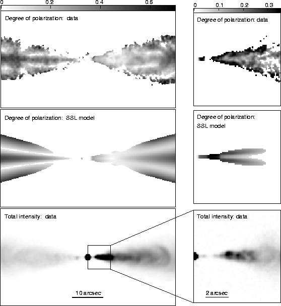
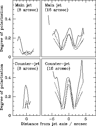
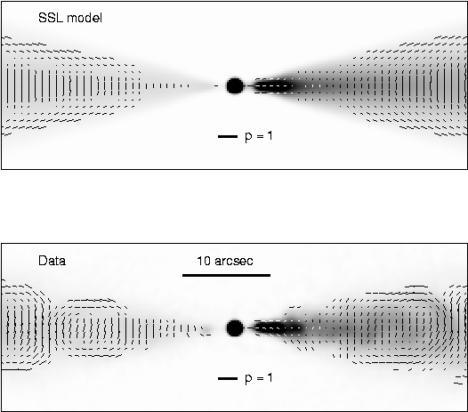
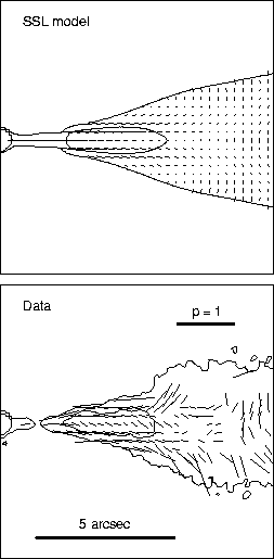
Fig. 12 shows the predicted and observed degrees of polarization $p = (Q^2+U^2)^{1/2}/I$ at both resolutions, with the I images below them for reference. The degree and direction of polarization are represented in Figs 13 and 14 by vectors whose magnitudes are proportional to the degree of polarization and whose directions are those of the apparent magnetic field (i.e. rotated by 90 $^\circ$ from the E-vector direction, after correcting the observations for Faraday rotation). 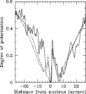Longitudinal and representative transverse profiles at the lower resolution are displayed in Figs 15 and 16, respectively.

**Figure 13:** Vectors whose lengths are proportional to the degree of polarization, p, and whose directions are those of the apparent magnetic field superimposed on grey-scale images of total intensity at 0.75 arcsec resolution. Top: spine/shear-layer model; bottom: VLA data. The vectors are blanked as in Fig. 12.
$\begin{figure}\epsfxsize =14cm \epsffile{overlay2.eps}\end{figure}$

**Figure 14:** Vectors whose lengths are proportional to the degree of polarization, p, and whose directions are those of the apparent magnetic field superimposed on contours of total intensity at 0.25arcsec resolution. Top: spine/shear-layer model; bottom: VLA data. The observed vectors are blanked on polarized and total intensity, as in Fig. 12, but the model vectors are plotted wherever the total intensity exceeds $5\sigma$ , regardless of polarized flux.
$\begin{figure}\epsfxsize =7cm \epsffile{pvect025.eps}\end{figure}$

**Figure 15:** Profile of the degree of polarization along the jet ridge line at 0.75 arcsec resolution. Full line: data; dashed line: spine/shear layer fit; dotted line: Gaussian fit.
$\begin{figure}\epsfxsize =8.5cm \epsffile{pprof.eps}\end{figure}$

**Figure 16:** Example transverse profiles of the degree of polarization at distances of 8arcsec from the core in the flaring region (left panels) and 16 arcsec from the core in the outer region (right panels). Top panels: main jet; bottom panel: counter-jet. Full line: data; dashed line: spine/shear-layer fit; dotted line: Gaussian fit. The profiles are blanked as in Fig. 12 and the resolution is 0.75 arcsec.
$\begin{figure}\epsfxsize =8.5cm \epsffile{ptran.eps}\end{figure}$