4.1.6 Features that cannot be fitted well

The models are in principle incapable of fitting non-axisymmetric or small-scale features. The most important examples of these, emphasized in the plots of $\chi ^2$ for Stokes I and U (Fig. 5) are as follows:

1. The inner and flaring regions of the main and counter-jets have fine structure consisting of small numbers of discrete knots. These are modelled as continuous features with the correct mean level (Fig. 9).
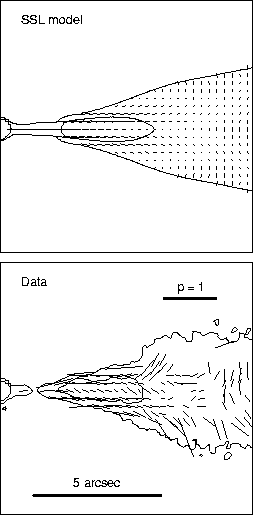
2. The observed apparent magnetic field direction is oblique to the jet axis in the centre of the flaring region of the main jet (Fig. 14): this cannot be reproduced in any purely axisymmetric model.
3. The prominent arc of emission 20 to 24arcsec from the nucleus in the main jet is not reproduced either in total intensity or linear polarization.

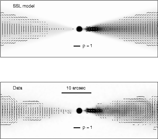
Figure 13: Vectors whose lengths are proportional to the degree of polarization, p, and whose directions are those of the apparent magnetic field superimposed on grey-scale images of total intensity at 0.75 arcsec resolution. Top: spine/shear-layer model; bottom: VLA data. The vectors are blanked as in Fig. 12.

Figure 14: Vectors whose lengths are proportional to the degree of polarization, p, and whose directions are those of the apparent magnetic field superimposed on contours of total intensity at 0.25 arcsec resolution. Top: spine/shear-layer model; bottom: VLA data. The observed vectors are blanked on polarized and total intensity, as in Fig. 12, but the model vectors are plotted wherever the total intensity exceeds $5\sigma$, regardless of polarized flux.

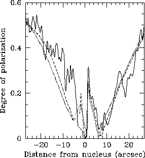
Figure 15: Profile of the degree of polarization along the jet ridge line at 0.75 arcsec resolution. Full line: data; dashed line: spine/shear layer fit; dotted line: Gaussian fit.

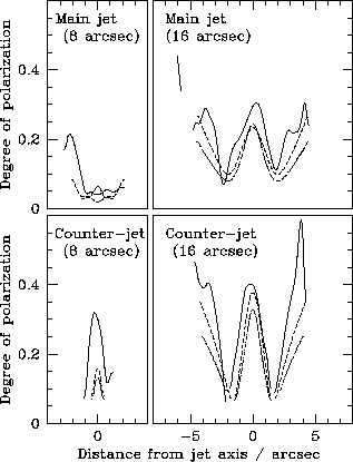
Figure 16: Example transverse profiles of the degree of polarization at distances of 8arcsec from the core in the flaring region (left panels) and 16arcsec from the core in the outer region (right panels). Top panels: main jet; bottom panel: counter-jet. Full line: data; dashed line: spine/shear-layer fit; dotted line: Gaussian fit. The profiles are blanked as in Fig. 12 and the resolution is 0.75arcsec.

In addition, there are small but significant deviations between observed and modelled polarization patterns in the flaring region:

1. The apparent field vectors between 5 and 7 arcsec from the nucleus in the main jet diverge more from the axis than is predicted (Fig. 14). The degree of polarization also appears to be underestimated, but the signal-to-noise ratio at 0.25 arcsec FWHM is quite low and that the observed vectors are blanked on polarized flux. There is therefore a tendency for the degree of polarization to be spuriously high for the plotted vectors. This effect has been corrected to first order (Section 2.3), but some residual remains.
2. The degree of polarization along the ridge-line of the counter-jet is underestimated, significantly so between 3 and 10 arcsec from the core (Figs 15 and 16).

2002-06-13